Note
Click here to download the full example code or to run this example in your browser via Binder
Sensor Platform Simulation Example
This example looks at how platforms and sensors can be used within the Stone Soup simulation capability.
Building a Simulated Sensor Platform
The focus of this example is to show how to setup and configure simulations, as such the application of a tracker will not be covered in detail. For more information about trackers and how to configure them review of the tutorials and demonstrations is recommended.
This example makes use of Stone Soup FixedPlatform and Sensor objects.
In order to configure platforms, sensors and the simulation we will need to import some specific Stone Soup objects. As these have been introduced in previous tutorials they are imported upfront. New functionality within this example will be imported at the relevant point in order to draw attention to the new features.
# Some general imports and set up
from datetime import datetime
from datetime import timedelta

import numpy as np

# Stone Soup imports:
from stonesoup.types.state import State, GaussianState
from stonesoup.types.array import StateVector, CovarianceMatrix
from stonesoup.models.transition.linear import (
    CombinedLinearGaussianTransitionModel, ConstantVelocity)
from stonesoup.models.measurement.nonlinear import CartesianToElevationBearingRange
from stonesoup.updater.kalman import UnscentedKalmanUpdater
from stonesoup.predictor.kalman import UnscentedKalmanPredictor
from stonesoup.deleter.time import UpdateTimeStepsDeleter
from stonesoup.tracker.simple import MultiTargetTracker
from matplotlib import pyplot as plt

# Define the simulation start time
start_time = datetime.now()
Create a Platform
The first element we need to create is a platform. For this first example we will build a static (or fixed) platform which is located at the origin. For this example we are going to work in a 6-dimensional state space our platform will have the following \(\mathbf{x}\).
Because the platform is static we only need to define \((x, y, z)\), any internal interaction with the platform which requires knowledge of platform velocity \((\dot{x}, \dot{y}, \dot{z})\) will be returned \((0, 0, 0)\).
# First import the fixed platform
from stonesoup.platform.base import FixedPlatform

# Define the initial platform position, in this case the origin
platform_state_vector = StateVector([[0], [0], [0]])
position_mapping = (0, 1, 2)

# Create the initial state (position, time), notice it is set to the simulation start time defined earlier
platform_state = State(platform_state_vector, start_time)

# create our fixed platform
platform = FixedPlatform(states=platform_state,
                         position_mapping=position_mapping)
We have now created a platform within Stone Soup and located it at the origin of our state space. As previously stated the platform will have a velocity \((\dot{x}, \dot{y}, \dot{z})\) of \((0, 0, 0)\) which we can check:
platform.velocity
StateVector([[0],
             [0],
             [0]])
We can also query the platform orientation:
platform.orientation
StateVector([[0],
             [0],
             [0]])
Create a Sensor
Now that we have a platform the next step is to create a sensor which can be added to the platform. In this example a Radar will be created which is capable of measuring the range, bearing and elevation of the target relative to the sensor.
The RadarRangeBearingElevation provides a sensor wrapper around the
CartesianToElevationBearingRange measurement model. The measurement model provides a time-invariant
measurement model, where measurements are assumed to be received in the form of elevation (\(\theta\)),
bearing (\(\phi\)) and range (\(r\)) with Gaussian noise in each dimension.
The model is described by the following equations:
where \(\mathbf{z}_k\) is a measurement vector of the form:
and \(h\) is a non-linear model function of the form:
and finally \(\mathbf{z}_k\) is Gaussian distributed with covariance \(R\), i.e.:
We now create our radar.
# Import a radar sensor model
from stonesoup.sensor.radar.radar import RadarElevationBearingRange

# First we need to configure a radar

# Generate a radar sensor with a suitable measurement accuracy
noise_covar = CovarianceMatrix(np.array(np.diag([np.deg2rad(3)**2,
                                                 np.deg2rad(0.15)**2,
                                                 25**2])))
# this radar measures range with an accuracy of +/- 25m, and elevation accuracy +/- 3
# degrees and bearing accuracy of +/- 0.15 degrees

# The radar needs to be informed of where x, y, and z are in the target state space
radar_mapping = (0, 2, 4)

# Instantiate the radar
radar = RadarElevationBearingRange(ndim_state=6,
                                   position_mapping=radar_mapping,
                                   noise_covar=noise_covar)
Attach the sensor to the platform
Now that we have created our radar sensor we need to mount the sensor onto the platform we have previously created.
Sensors can be mounted with two additional parameters; the mounting offset and rotation offset.
The mounting offset:
defines how the sensors position is offset from the platform,
defaults to a position offset of zero.
The rotation_offset:
defines the sensors orientation relative to that of the platform,
defaults to a zero orientation offset.
The default assumption is that the sensor is located at the centre point of the platform and orientated to align with the platform body. In this example we are happy to use the default assumptions and therefore the sensor can be added.
platform.add_sensor(radar)
As before we can query the platform to demonstrate that it has a sensor mounted:
(RadarElevationBearingRange(
    position_mapping=(0, 2, 4),
    noise_covar=CovarianceMatrix([[2.74155678e-03, 0.00000000e+00, 0.00000000e+00],
                                  [0.00000000e+00, 6.85389195e-06, 0.00000000e+00],
                                  [0.00000000e+00, 0.00000000e+00, 6.25000000e+02]]),
    resolutions=None,
    rotation_offset=StateVector([[0],
                                 [0],
                                 [0]]),
    mounting_offset=StateVector([[0],
                                 [0],
                                 [0]]),
    movement_controller=FixedMovable(
                            states=[State(
                                       state_vector=StateVector([[0],
                                                                 [0],
                                                                 [0]]),
                                       timestamp=2022-10-10 15:57:32.485261)],
                            position_mapping=(0, 1, 2),
                            velocity_mapping=None,
                            orientation=StateVector([[0],
                                                     [0],
                                                     [0]])),
    clutter_model=None,
    ndim_state=6,
    max_range=inf),)
You will notice that platform.sensors returns a list which contains our single sensor. This hints at the multi-sensor platform functionality which is shown in a subsequent example.
We can also check to ensure that the default mounting_offsets have been applied:
StateVector([[0],
             [0],
             [0]])
And that the rotation_offsets have been applied:
StateVector([[0],
             [0],
             [0]])
Building a simulation
Now that we have created a sensor platform we need to build a simulation which generates targets for the sensor to
detect and track. For this example we are going to use a MultiTargetGroundTruthSimulator. this simulator
enables multiple ground truth targets to be created based on a number of user defined parameters.
In this example targets are initiated with values based upon a mean state and a covariance, using a Gaussian
assumption. This is done by creating a GaussianState object which describes the distribution from which we
want our targets to be drawn from. For this example targets will be generated using the following parameters:
\(x\) is Gaussian distributed around the platform location with variance of \(\mathrm{2}km\)
\(y\) is Gaussian distributed around the platform location with variance of \(\mathrm{2}km\)
\(z\) is Gaussian distributed around an altitude of \(\mathrm{9}km\) with variance of \(\mathrm{0.1}km\)
\(\dot{x}\) is Gaussian distributed around \(\mathrm{100}ms^{-1}\) with variance of \(\mathrm{50}ms^{-1}\)
\(\dot{y}\) is Gaussian distributed around \(\mathrm{100}ms^{-1}\) with variance of \(\mathrm{50}ms^{-1}\)
\(\dot{z}\) is Gaussian distributed around \(\mathrm{0}ms^{-1}\) with variance of \(\mathrm{1}ms^{-1}\)
We will also configure our simulator to randomly create and delete targets, based on a birth rate and death rate we specify. In this example we set the birth rate to be 0.10, i.e. on any given time step there is a 10% chance of a new target being initiated. We have set the death rate to 0.01, i.e. on any given time step there is a 1% chance that a target will be removed from the simulation.
The above setup will provide a case which loosely approximates an air surveillance radar at an airport.
from stonesoup.simulator.simple import MultiTargetGroundTruthSimulator

# Set a constant velocity transition model for the targets
transition_model = CombinedLinearGaussianTransitionModel(
    [ConstantVelocity(0.5), ConstantVelocity(0.5), ConstantVelocity(0.1)])

# Define the Gaussian State from which new targets are sampled on initialisation
initial_target_state = GaussianState(StateVector([[0], [0], [0], [0], [9000], [0]]),
                                     CovarianceMatrix(np.diag([2000, 50, 2000, 50, 100, 1])))

groundtruth_sim = MultiTargetGroundTruthSimulator(
    transition_model=transition_model,  # target transition model
    initial_state=initial_target_state,  # add our initial state for targets
    timestep=timedelta(seconds=1),  # time between measurements
    number_steps=120,  # 2 minute
    birth_rate=0.10,  # 10% chance of a new target being born
    death_probability=0.01  # 1% chance of a target being killed
)
Now that we have set up our ground truth simulation we need to add our platform into the simulation capability. This
is done using the PlatformDetectionSimulator. This simulator allows a list of platforms to be added into
the simulation, when the simulation is processed the platforms are able to make detections of both the ground truth
targets and other platforms.
In this case we have a single platform, therefore the radar sensor on this platform will only be able to make measurements of the ground truth objects generated by the simulator.
# Import the PlatformDetectionSimulator
from stonesoup.simulator.platform import PlatformDetectionSimulator

sim = PlatformDetectionSimulator(groundtruth=groundtruth_sim, platforms=[platform])
Creating the Tracker Components
As stated above the aim of this example is to show how Platform, Sensor and
Simulator work within Stone Soup. We will therefore quickly build an Unscented Kalman Filter which
initiates measurements using a simple heuristic initiation and deletes any track where no detection is associated for
2 consecutive time steps. There are a number of tutorials for how to build the tracking components provided in the
Tutorials.
# Create an Unscented Kalman Predictor
predictor = UnscentedKalmanPredictor(transition_model)

# Create an Unscented Kalman Updater, note our sensor adds a measurement model to detections
updater = UnscentedKalmanUpdater(measurement_model=None)
When we build our updater you will notice that we do not provide a measurement model. This is because we
have defined a measurement model which is attached to our radar sensor, each detection made by this sensor
will have our radar measurement model associated with it. In Stone Soup the Updater checks the
detections provided and will use any measurement model attached to the detection.
Setup Initiator class for the Tracker
We will now build a simple heuristic initiator. This assumes most of the deviation is caused by the bearing measurement error. It converts the bearing error error into \(x, y\) components using the target bearing. For z, we simply use \(r*\sigma_{\theta}^2\) (this ignores any bearing or range related components). Velocity covariances are just based on expected velocity range of targets.
from stonesoup.types.state import GaussianState
from stonesoup.types.update import GaussianStateUpdate
from stonesoup.initiator.simple import SimpleMeasurementInitiator
from stonesoup.types.track import Track
from stonesoup.types.hypothesis import SingleHypothesis


class Initiator(SimpleMeasurementInitiator):
    def initiate(self, detections, timestamp, **kwargs):
        MAX_DEV = 500.
        tracks = set()
        measurement_model = self.measurement_model
        for detection in detections:
            state_vector = measurement_model.inverse_function(
                            detection)
            model_covar = measurement_model.covar()

            el_az_range = np.sqrt(np.diag(model_covar))  # elev, az, range

            std_pos = detection.state_vector[2, 0]*el_az_range[1]
            stdx = np.abs(std_pos*np.sin(el_az_range[1]))
            stdy = np.abs(std_pos*np.cos(el_az_range[1]))
            stdz = np.abs(detection.state_vector[2, 0]*el_az_range[0])
            if stdx > MAX_DEV:
                print('Warning - X Deviation exceeds limit!!')
            if stdy > MAX_DEV:
                print('Warning - Y Deviation exceeds limit!!')
            if stdz > MAX_DEV:
                print('Warning - Z Deviation exceeds limit!!')
            C0 = np.diag(np.array([stdx, 50.0, stdy, 50.0, stdz, 10.0])**2)

            tracks.add(Track([GaussianStateUpdate(
                state_vector,
                C0,
                SingleHypothesis(None, detection),
                timestamp=detection.timestamp)
            ]))
        return tracks


meas_model = CartesianToElevationBearingRange(
            ndim_state=6,
            mapping=np.array([0, 2, 4]),
            noise_covar=noise_covar)

prior_state = GaussianState(
        np.array([[0], [0], [0], [0], [0], [0]]),
        np.diag([1000, 50, 1000, 50, 1000, 10.0])**2)

initiator = Initiator(prior_state, measurement_model=meas_model)
Now that we have setup out tracking scenario we can wrap our simulation environment within a
MultiTargetTracker. This takes our tracker configurations and the simulation we previously created and
brings them together into a single iterable object.
from stonesoup.hypothesiser.distance import DistanceHypothesiser
from stonesoup.measures import Mahalanobis
hypothesiser = DistanceHypothesiser(predictor, updater, measure=Mahalanobis(), missed_distance=3)

from stonesoup.dataassociator.neighbour import NearestNeighbour
data_associator = NearestNeighbour(hypothesiser)

deleter = UpdateTimeStepsDeleter(time_steps_since_update=2)

# Create a Kalman multi-target tracker
kalman_tracker = MultiTargetTracker(
    initiator=initiator,
    deleter=deleter,
    detector=sim,
    data_associator=data_associator,
    updater=updater
)
The final step is to iterate our tracker over the simulation:
kalman_tracks = {}  # Store for plotting later
groundtruth_paths = {}  # Store for plotting later
detections = []  # Store for plotting later

for time, ctracks in kalman_tracker:
    for track in ctracks:
        loc = (track.state_vector[0], track.state_vector[2])
        if track not in kalman_tracks:
            kalman_tracks[track] = []
        kalman_tracks[track].append(loc)

    for truth in groundtruth_sim.current[1]:
        loc = (truth.state_vector[0], truth.state_vector[2])
        if truth not in groundtruth_paths:
            groundtruth_paths[truth] = []
        groundtruth_paths[truth].append(loc)

    for detection in sim.detections:
        detect_state = detection.measurement_model.inverse_function(detection)
        loc = (detect_state[0], detect_state[2])
        detections.append(loc)
Warning - Z Deviation exceeds limit!!
Warning - Z Deviation exceeds limit!!
Warning - Z Deviation exceeds limit!!
Warning - Z Deviation exceeds limit!!
Warning - Z Deviation exceeds limit!!
Warning - Z Deviation exceeds limit!!
Warning - Z Deviation exceeds limit!!
Plotting the outputs
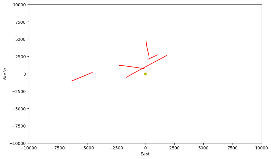
First we will plot the ground truth paths (red) which have been generated in the simulation step.
fig = plt.figure(figsize=(10, 6))
ax = fig.add_subplot(1, 1, 1)
ax.set_xlabel("$East$")
ax.set_ylabel("$North$")
ax.set_ylim(-10000, 10000)
ax.set_xlim(-10000, 10000)

for key in groundtruth_paths:
    X = [coord[0] for coord in groundtruth_paths[key]]
    Y = [coord[1] for coord in groundtruth_paths[key]]
    ax.plot(X, Y, color='r')  # Plot true locations in red

# plot platform location
ax.scatter(0, 0, color='y')
<matplotlib.collections.PathCollection object at 0x7f1b7c3c9540>
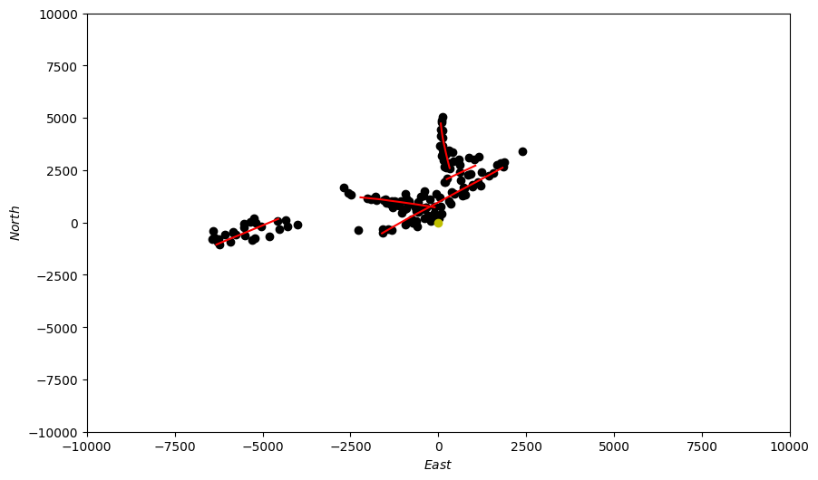
If we now overlay the detections (black) onto the ground truth paths (red) we can see how the sensor performs,
generating detections based upon the MeasurementModel we provided it with. The platform location is
shown in yellow.
fig = plt.figure(figsize=(10, 6))
ax = fig.add_subplot(1, 1, 1)
ax.set_xlabel("$East$")
ax.set_ylabel("$North$")
ax.set_ylim(-10000, 10000)
ax.set_xlim(-10000, 10000)

for key in groundtruth_paths:
    X = [coord[0] for coord in groundtruth_paths[key]]
    Y = [coord[1] for coord in groundtruth_paths[key]]
    ax.plot(X, Y, color='r')  # Plot true locations in red

X = [coord[0] for coord in detections]
Y = [coord[1] for coord in detections]
ax.scatter(X, Y, color='k')  # Plot detections in black

# plot platform location
ax.scatter(0, 0, color='y')
<matplotlib.collections.PathCollection object at 0x7f1b7bfe2ad0>
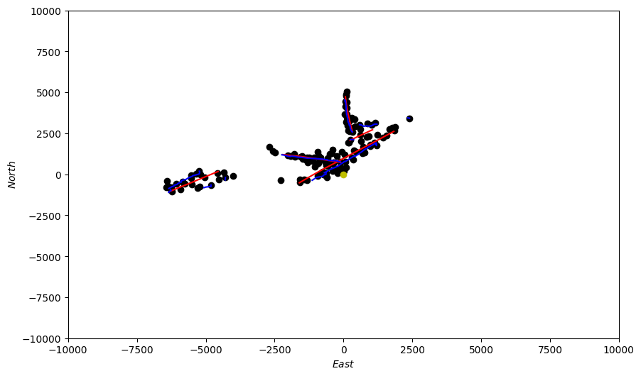
Now we overlay the ground truth locations (red), detections (black) and tracks (blue). This shows all the stages of the tracker simulation we have built in a single figure. The platform location is shown in yellow.
fig = plt.figure(figsize=(10, 6))
ax = fig.add_subplot(1, 1, 1)
ax.set_xlabel("$East$")
ax.set_ylabel("$North$")
ax.set_ylim(-10000, 10000)
ax.set_xlim(-10000, 10000)
for key in groundtruth_paths:
    X = [coord[0] for coord in groundtruth_paths[key]]
    Y = [coord[1] for coord in groundtruth_paths[key]]
    ax.plot(X, Y, color='r')  # Plot true locations in red

for key in kalman_tracks:
    X = [coord[0] for coord in kalman_tracks[key]]
    Y = [coord[1] for coord in kalman_tracks[key]]
    ax.plot(X, Y, color='b')  # Plot track estimates in blue

X = [coord[0] for coord in detections]
Y = [coord[1] for coord in detections]
ax.scatter(X, Y, color='k')  # Plot detections in black

# plot platform location
ax.scatter(0, 0, color='y')
<matplotlib.collections.PathCollection object at 0x7f1b7c05bee0>
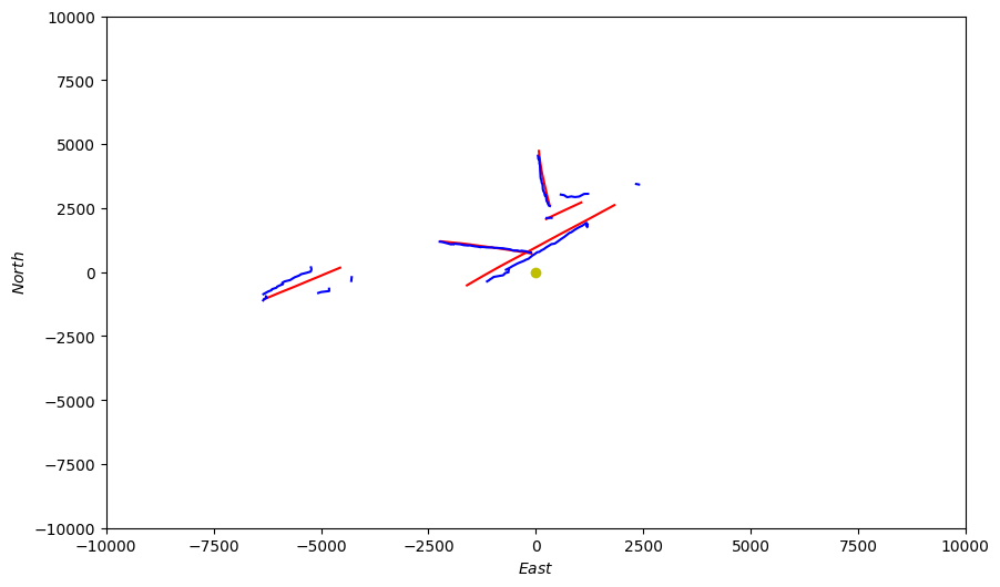
Finally, we can plot the estimated tracks (blue) alongside the ground truth paths (red). Because we used a noisy sensor this view makes it easier to quickly see the tracker performance. The platform location is shown in yellow.
fig = plt.figure(figsize=(10, 6))
ax = fig.add_subplot(1, 1, 1)
ax.set_xlabel("$East$")
ax.set_ylabel("$North$")
ax.set_ylim(-10000, 10000)
ax.set_xlim(-10000, 10000)
for key in groundtruth_paths:
    X = [coord[0] for coord in groundtruth_paths[key]]
    Y = [coord[1] for coord in groundtruth_paths[key]]
    ax.plot(X, Y, color='r')  # Plot true locations in red

for key in kalman_tracks:
    X = [coord[0] for coord in kalman_tracks[key]]
    Y = [coord[1] for coord in kalman_tracks[key]]
    ax.plot(X, Y, color='b')  # Plot track estimates in blue

# plot platform location
ax.scatter(0, 0, color='y')
<matplotlib.collections.PathCollection object at 0x7f1b7bf5f4c0>
To familiarise yourself with sensors it is recommended that you investigate changing the parameters within the sensor
Measurement Model in order to see the impact on detections and ultimately tracker performance. For this example we
used a hard association logic coupled with a relatively noisy sensor. A suggested further exercise is to modify this
example to use a soft association step such as Probabilistic Data Association (PDA) or
Joint Probabilistic Data Association (JPDA).
Key points
Sensor platforms, which combine
SensorandPlatformcan be created in Stone Soup and used as part of a tracking simulation.When using a
Sensorto generate detections there is no need to provide anUpdaterwith aMeasurementModelas each detection is attributed with the relevant sensors measurement model.Sensors will generate detections of all platforms within the simulation, not just ground truth objects.
Total running time of the script: ( 0 minutes 3.080 seconds)