3 - Avoiding Data Incest

Introduction

This tutorial uses the Stone Soup architecture module to provide an example of how data incest can occur in a poorly designed network.

In this example, data incest is shown in a simple architecture. A top-level fusion node receives data from two sources, which contain information (tracks) sourced from two sensors. However, one sensor is overly represented, due to a triangle in the information architecture graph. As a consequence, the fusion node becomes overconfident, or biased towards the duplicated data.

The aim is to demonstrate this effect by modelling two similar information architectures: a centralised (non-hierarchical) architecture, and a hierarchical alternative, and looks to compare the fused results at the top-level node.

We will follow the following steps:

1. Define sensors for sensor nodes

2. Simulate a ground truth, as a basis for the simulation

3. Create trackers for fusion nodes

4. Build a non-hierarchical architecture, containing a triangle

5. Build a hierarchical architecture by removing an edge from the non-hierarchical architecture

6. Compare and contrast. What difference, if any, will the hierarchical alternative make?

import random
import copy
import math
import numpy as np
import matplotlib.pyplot as plt
from datetime import datetime, timedelta

start_time = datetime.now().replace(microsecond=0)
np.random.seed(1990)
random.seed(1990)

1) Sensors

We need two sensors to be assigned to the two sensor nodes. Notice they vary only in their position.

from stonesoup.models.clutter import ClutterModel
from stonesoup.models.measurement.linear import LinearGaussian
from stonesoup.types.state import CovarianceMatrix

mm = LinearGaussian(ndim_state=4,
                    mapping=[0, 2],
                    noise_covar=CovarianceMatrix(np.diag([0.5, 0.5])),
                    seed=6)

mm2 = LinearGaussian(ndim_state=4,
                     mapping=[0, 2],
                     noise_covar=CovarianceMatrix(np.diag([0.5, 0.5])),
                     seed=6)

from stonesoup.sensor.sensor import SimpleSensor
from stonesoup.models.measurement.base import MeasurementModel
from stonesoup.base import Property


class DummySensor(SimpleSensor):
    measurement_model: MeasurementModel = Property(doc=":class:`~.MeasurementModel` to be used")

    def is_detectable(self, *args, **kwargs):
        return True

    def is_clutter_detectable(self, *args, **kwargs):
        return True


sensor1 = DummySensor(measurement_model=mm,
                      position=np.array([[10], [-20]]),
                      clutter_model=ClutterModel(clutter_rate=5,
                                                 dist_params=((-100, 100), (-50, 60)), seed=6))
sensor1.clutter_model.distribution = sensor1.clutter_model.random_state.uniform
sensor2 = DummySensor(measurement_model=mm2,
                      position=np.array([[10], [20]]),
                      clutter_model=ClutterModel(clutter_rate=5,
                                                 dist_params=((-100, 100), (-50, 60)), seed=6))
sensor2.clutter_model.distribution = sensor2.clutter_model.random_state.uniform

2) Ground Truth

from stonesoup.models.transition.linear import CombinedLinearGaussianTransitionModel, \
    ConstantVelocity
from stonesoup.types.groundtruth import GroundTruthPath, GroundTruthState
from ordered_set import OrderedSet

# Generate transition model
transition_model = CombinedLinearGaussianTransitionModel([ConstantVelocity(0.005),
                                                          ConstantVelocity(0.005)])

yps = range(0, 100, 10)  # y value for prior state
truths = OrderedSet()
ntruths = 3  # number of ground truths in simulation
time_max = 60  # timestamps the simulation is observed over
timesteps = [start_time + timedelta(seconds=k) for k in range(time_max)]

xdirection = 1
ydirection = 1

# Generate ground truths
for j in range(0, ntruths):
    truth = GroundTruthPath([GroundTruthState([0, xdirection, yps[j], ydirection],
                                              timestamp=timesteps[0])], id=f"id{j}")

    for k in range(1, time_max):
        truth.append(
            GroundTruthState(transition_model.function(truth[k - 1], noise=True,
                                                       time_interval=timedelta(seconds=1)),
                             timestamp=timesteps[k]))
    truths.add(truth)

    xdirection *= -1
    if j % 2 == 0:
        ydirection *= -1

3) Build Trackers

We use the same configuration of trackers and track-trackers as we did in the previous tutorial.

from stonesoup.predictor.kalman import KalmanPredictor
from stonesoup.updater.kalman import ExtendedKalmanUpdater
from stonesoup.hypothesiser.distance import DistanceHypothesiser
from stonesoup.measures import Mahalanobis
from stonesoup.dataassociator.neighbour import GNNWith2DAssignment
from stonesoup.deleter.error import CovarianceBasedDeleter
from stonesoup.types.state import GaussianState
from stonesoup.initiator.simple import MultiMeasurementInitiator
from stonesoup.tracker.simple import MultiTargetTracker
from stonesoup.architecture.edge import FusionQueue

prior = GaussianState([[0], [1], [0], [1]], np.diag([1, 1, 1, 1]))
predictor = KalmanPredictor(transition_model)
updater = ExtendedKalmanUpdater(measurement_model=None)
hypothesiser = DistanceHypothesiser(predictor, updater, measure=Mahalanobis(), missed_distance=5)
data_associator = GNNWith2DAssignment(hypothesiser)
deleter = CovarianceBasedDeleter(covar_trace_thresh=3)
initiator = MultiMeasurementInitiator(
    prior_state=prior,
    measurement_model=None,
    deleter=deleter,
    data_associator=data_associator,
    updater=updater,
    min_points=5,
)

tracker = MultiTargetTracker(initiator, deleter, None, data_associator, updater)

Track Tracker

from stonesoup.updater.wrapper import DetectionAndTrackSwitchingUpdater
from stonesoup.updater.chernoff import ChernoffUpdater
from stonesoup.feeder.track import Tracks2GaussianDetectionFeeder

track_updater = ChernoffUpdater(None)
detection_updater = ExtendedKalmanUpdater(None)
detection_track_updater = DetectionAndTrackSwitchingUpdater(None, detection_updater, track_updater)

fq = FusionQueue()

track_tracker = MultiTargetTracker(
    initiator, deleter, None, data_associator, detection_track_updater)

4) Non-Hierarchical Architecture

We start by constructing the non-hierarchical, centralised architecture.

Nodes

from stonesoup.architecture.node import SensorNode, FusionNode

sensornode1 = SensorNode(sensor=copy.deepcopy(sensor1), label='Sensor Node 1')
sensornode1.sensor.clutter_model.distribution = \
    sensornode1.sensor.clutter_model.random_state.uniform

sensornode2 = SensorNode(sensor=copy.deepcopy(sensor2), label='Sensor Node 2')
sensornode2.sensor.clutter_model.distribution = \
    sensornode2.sensor.clutter_model.random_state.uniform

f1_tracker = copy.deepcopy(track_tracker)
f1_fq = FusionQueue()
f1_tracker.detector = Tracks2GaussianDetectionFeeder(f1_fq)
fusion_node1 = FusionNode(tracker=f1_tracker, fusion_queue=f1_fq, label='Fusion Node 1')

f2_tracker = copy.deepcopy(track_tracker)
f2_fq = FusionQueue()
f2_tracker.detector = Tracks2GaussianDetectionFeeder(f2_fq)
fusion_node2 = FusionNode(tracker=f2_tracker, fusion_queue=f2_fq, label='Fusion Node 2')

Edges

Here we define the set of edges for the non-hierarchical (NH) architecture.

from stonesoup.architecture import InformationArchitecture
from stonesoup.architecture.edge import Edge, Edges

NH_edges = Edges([Edge((sensornode1, fusion_node1), edge_latency=0),
                  Edge((sensornode1, fusion_node2), edge_latency=0),
                  Edge((sensornode2, fusion_node2), edge_latency=0),
                  Edge((fusion_node2, fusion_node1), edge_latency=0)])

Create the Non-Hierarchical Architecture

The cell below should create and plot the architecture we have built. This architecture is at risk of data incest, due to the fact that information from sensor node 1 could reach Fusion Node 1 via two routes, while appearing to not be from the same source:

• Route 1: Sensor Node 1 (S1) passes its information straight to Fusion Node 1 (F1)

• Route 2: S1 also passes its information to Fusion Node 2 (F2). Here it is fused with information from Sensor Node 2 (S2). This resulting information is then passed to Fusion Node 1.

Ultimately, F1 is recieving information from S1, and information from F2 which is based on the same information from S1. This can cause a bias towards the information created at S1. In this example, we would expect to see overconfidence in the form of unrealistically small uncertainty of the output tracks.

NH_architecture = InformationArchitecture(NH_edges, current_time=start_time,
                                          use_arrival_time=True)
NH_architecture

Run the Non-Hierarchical Simulation

for time in timesteps:
    NH_architecture.measure(truths, noise=True)
    NH_architecture.propagate(time_increment=1)

Extract all Detections that arrived at Non-Hierarchical Node C

NH_sensors = []
NH_dets = set()
for sn in NH_architecture.sensor_nodes:
    NH_sensors.append(sn.sensor)
    for timestep in sn.data_held['created'].keys():
        for datapiece in sn.data_held['created'][timestep]:
            NH_dets.add(datapiece.data)

Plot the tracks stored at Non-Hierarchical Node C

from stonesoup.plotter import Plotterly


def reduce_tracks(tracks):
    return {
        type(track)([s for s in track.last_timestamp_generator()])
        for track in tracks}


plotter = Plotterly()
plotter.plot_ground_truths(truths, [0, 2])
plotter.plot_measurements(NH_dets, [0, 2])
for node in NH_architecture.fusion_nodes:
    hexcol = ["#" + ''.join([random.choice('ABCDEF0123456789') for i in range(6)])]
    plotter.plot_tracks(reduce_tracks(node.tracks), [0, 2], track_label=str(node.label),
                        line=dict(color=hexcol[0]), uncertainty=True)
plotter.plot_sensors(NH_sensors)
plotter.fig

5) Hierarchical Architecture

We now create an alternative architecture. We recreate the same set of nodes as before, but with a new edge set, which is a subset of the edge set used in the non-hierarchical architecture.

In this architecture, by removing the edge joining sensor node 1 to fusion node 2, we prevent data incest by removing the second path which data from sensor node 1 can take to reach fusion node 1.

Regenerate nodes identical to those in the non-hierarchical example

from stonesoup.architecture.node import SensorNode, FusionNode

sensornode1B = SensorNode(sensor=copy.deepcopy(sensor1), label='Sensor Node 1')
sensornode1B.sensor.clutter_model.distribution = \
    sensornode1B.sensor.clutter_model.random_state.uniform

sensornode2B = SensorNode(sensor=copy.deepcopy(sensor2), label='Sensor Node 2')
sensornode2B.sensor.clutter_model.distribution = \
    sensornode2B.sensor.clutter_model.random_state.uniform

f1_trackerB = copy.deepcopy(track_tracker)
f1_fqB = FusionQueue()
f1_trackerB.detector = Tracks2GaussianDetectionFeeder(f1_fqB)
fusion_node1B = FusionNode(tracker=f1_trackerB, fusion_queue=f1_fqB, label='Fusion Node 1')

f2_trackerB = copy.deepcopy(track_tracker)
f2_fqB = FusionQueue()
f2_trackerB.detector = Tracks2GaussianDetectionFeeder(f2_fqB)
fusion_node2B = FusionNode(tracker=f2_trackerB, fusion_queue=f2_fqB, label='Fusion Node 2')

Create Edges forming a Hierarchical Architecture

H_edges = Edges([Edge((sensornode1B, fusion_node1B), edge_latency=0),
                 Edge((sensornode2B, fusion_node2B), edge_latency=0),
                 Edge((fusion_node2B, fusion_node1B), edge_latency=0)])

Create the Hierarchical Architecture

The only difference between the two architectures is the removal of the edge from Sensor Node 1 to Fusion Node 2. This change removes the second route for information to travel from Sensor Node 1 to Fusion Node 1.

H_architecture = InformationArchitecture(H_edges, current_time=start_time,
                                         use_arrival_time=True)
H_architecture

Run the Hierarchical Simulation

for time in timesteps:
    H_architecture.measure(truths, noise=True)
    H_architecture.propagate(time_increment=1)

Extract all detections that arrived at Hierarchical Node C

H_sensors = []
H_dets = set()
for sn in H_architecture.sensor_nodes:
    H_sensors.append(sn.sensor)
    for timestep in sn.data_held['created'].keys():
        for datapiece in sn.data_held['created'][timestep]:
            H_dets.add(datapiece.data)

Plot the tracks stored at Hierarchical Node C

plotter = Plotterly()
plotter.plot_ground_truths(truths, [0, 2])
plotter.plot_measurements(H_dets, [0, 2])
for node in H_architecture.fusion_nodes:
    hexcol = ["#" + ''.join([random.choice('ABCDEF0123456789') for i in range(6)])]
    plotter.plot_tracks(reduce_tracks(node.tracks), [0, 2], track_label=str(node.label),
                        line=dict(color=hexcol[0]), uncertainty=True)
plotter.plot_sensors(H_sensors)
plotter.fig

Metrics

At a glance, the results from the hierarchical architecture look similar to the results from the original centralised architecture. We will now calculate and plot some metrics to give an insight into the differences.

Trace of Covariance Matrix

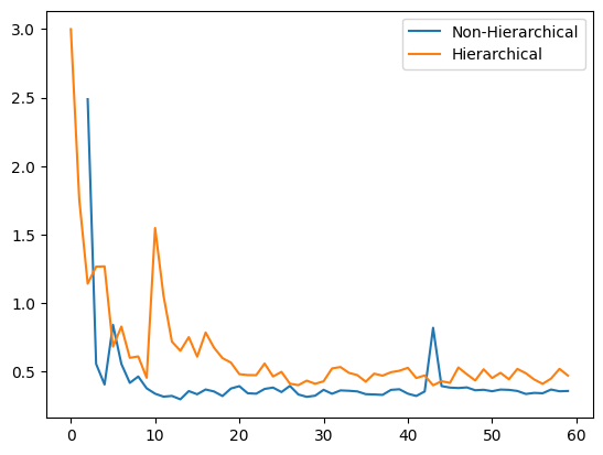
A consequence of data incest in tracking is overconfidence in track states. In this example we would expect to see unrealistically small uncertainty in the tracks generated by Fusion Node 1 in the non-hierarchical architecture.

To investigate this, we plot the mean trace of the covariance matrix of track states at each time step – for both architectures. We should expect to see that the uncertainty of the non-hierarchical architecture is lower than the hierarchical architecture, despite both receiving an identical set of measurements.

NH_tracks = [node.tracks for node in
             NH_architecture.fusion_nodes if node.label == 'Fusion Node 1'][0]
H_tracks = [node.tracks for node in
            H_architecture.fusion_nodes if node.label == 'Fusion Node 1'][0]

NH_mean_covar_trace = []
H_mean_covar_trace = []

for t in timesteps:
    NH_states = sum([[state for state in track.states if state.timestamp == t] for track in
                     NH_tracks], [])
    H_states = sum([[state for state in track.states if state.timestamp == t] for track in
                    H_tracks], [])

    if NH_states:
        NH_trace_mean = np.mean([np.trace(s.covar) for s in NH_states])
        NH_mean_covar_trace.append(NH_trace_mean)
    else:
        NH_mean_covar_trace.append(np.nan)

    if H_states:
        H_trace_mean = np.mean([np.trace(s.covar) for s in H_states])
        H_mean_covar_trace.append(H_trace_mean if not math.isnan(H_trace_mean) else 0)
    else:
        H_mean_covar_trace.append(np.nan)

As expected, the plot shows that the non-hierarchical architecture has a lower mean covariance trace. A naive observer may think this makes it higher performing, but we know that in fact it is a sign of overconfidence.

plt.plot(NH_mean_covar_trace, label="Non-Hierarchical")
plt.plot(H_mean_covar_trace, label="Hierarchical")
plt.legend(loc="upper right")
plt.show()