Note
Go to the end to download the full example code or to run this example in your browser via Binder.
7 - Probabilistic data association tutorial
Making an assignment between a single track and a single measurement can be problematic. In the previous tutorials you may have encountered the phenomenon of track seduction. This occurs when clutter, or other track, points are mis-associated with a prediction. If this happens repeatedly (as can be the case in high-clutter or low-\(p_d\) situations) the track can deviate significantly from the truth.
Rather than make a firm assignment at each time-step, we could work out the probability that each measurement should be assigned to a particular target. We could then propagate a measure of these collective probabilities to mitigate the effect of track seduction.
Pictorially:
Calculate a posterior for each hypothesis;
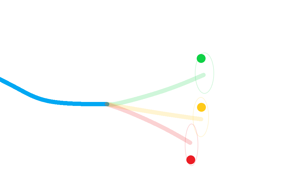
Weight each posterior state according to the probability that its corresponding hypothesis was true (including the probability of missed-detection);
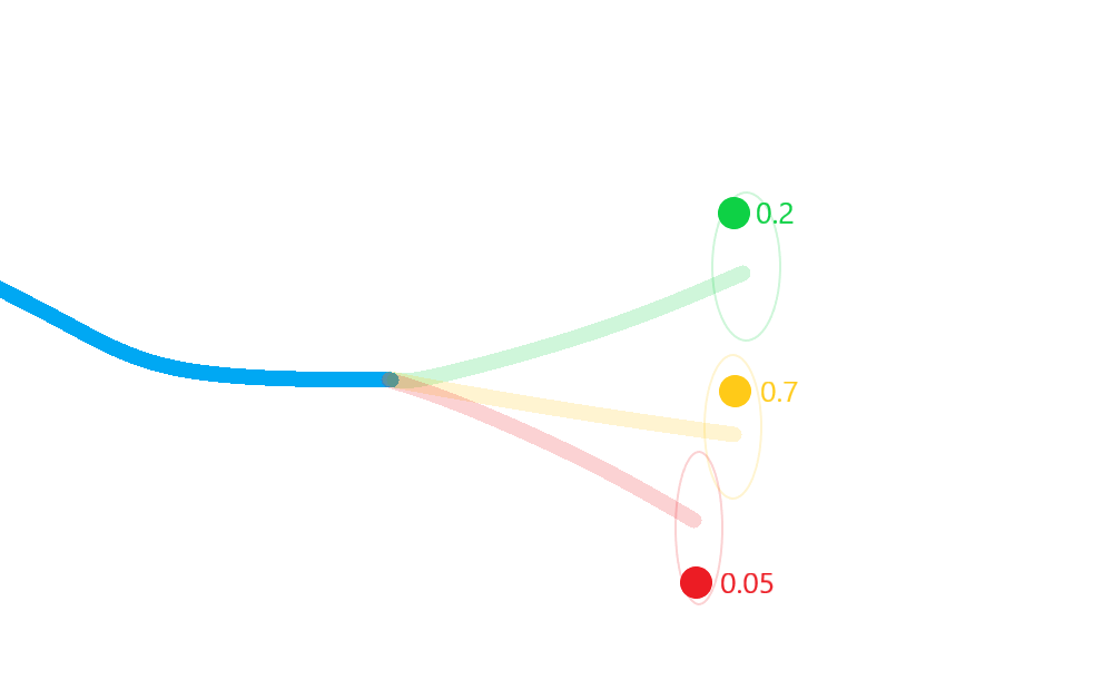
Merge the resulting estimate states in to a single posterior approximation.
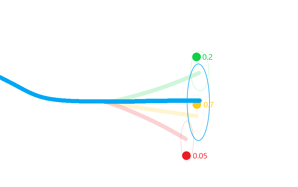
This results in a more robust approximation to the posterior state covariances that incorporates not only the uncertainty in state, but also in the association.
A PDA filter example
Ground truth
So, as before, we’ll first begin by simulating some ground truth.
import numpy as np

from datetime import datetime
from datetime import timedelta

from stonesoup.models.transition.linear import CombinedLinearGaussianTransitionModel, \
                                               ConstantVelocity
from stonesoup.types.groundtruth import GroundTruthPath, GroundTruthState

np.random.seed(1991)

start_time = datetime.now().replace(microsecond=0)
transition_model = CombinedLinearGaussianTransitionModel([ConstantVelocity(0.005),
                                                          ConstantVelocity(0.005)])
timesteps = [start_time]
truth = GroundTruthPath([GroundTruthState([0, 1, 0, 1], timestamp=timesteps[0])])
for k in range(1, 21):
    timesteps.append(start_time+timedelta(seconds=k))
    truth.append(GroundTruthState(
        transition_model.function(truth[k-1], noise=True, time_interval=timedelta(seconds=1)),
        timestamp=timesteps[k]))
Add clutter.
from scipy.stats import uniform

from stonesoup.types.detection import TrueDetection
from stonesoup.types.detection import Clutter
from stonesoup.models.measurement.linear import LinearGaussian
measurement_model = LinearGaussian(
    ndim_state=4,
    mapping=(0, 2),
    noise_covar=np.array([[0.75, 0],
                          [0, 0.75]])
    )

prob_detect = 0.9  # 90% chance of detection.

all_measurements = []
for state in truth:
    measurement_set = set()

    # Generate detection.
    if np.random.rand() <= prob_detect:
        measurement = measurement_model.function(state, noise=True)
        measurement_set.add(TrueDetection(state_vector=measurement,
                                          groundtruth_path=truth,
                                          timestamp=state.timestamp,
                                          measurement_model=measurement_model))

    # Generate clutter.
    truth_x = state.state_vector[0]
    truth_y = state.state_vector[2]
    for _ in range(np.random.randint(10)):
        x = uniform.rvs(truth_x - 10, 20)
        y = uniform.rvs(truth_y - 10, 20)
        measurement_set.add(Clutter(np.array([[x], [y]]), timestamp=state.timestamp,
                                    measurement_model=measurement_model))

    all_measurements.append(measurement_set)
Plot the ground truth and measurements with clutter.
from stonesoup.plotter import AnimatedPlotterly
plotter = AnimatedPlotterly(timesteps, tail_length=0.3)
plotter.plot_ground_truths(truth, [0, 2])

# Plot true detections and clutter.
plotter.plot_measurements(all_measurements, [0, 2])
plotter.fig
Create the predictor and updater
from stonesoup.predictor.kalman import KalmanPredictor
predictor = KalmanPredictor(transition_model)

from stonesoup.updater.kalman import KalmanUpdater
updater = KalmanUpdater(measurement_model)
Initialise Probabilistic Data Associator
The PDAHypothesiser and PDA associator generate track predictions and
calculate probabilities for all prediction-detection pairs for a single prediction and multiple
detections.
The PDAHypothesiser returns a collection of SingleProbabilityHypothesis
types. The PDA takes these hypotheses and returns a dictionary of key-value pairings
of each track and detection which it is to be associated with.
from stonesoup.hypothesiser.probability import PDAHypothesiser
hypothesiser = PDAHypothesiser(predictor=predictor,
                               updater=updater,
                               clutter_spatial_density=0.125,
                               prob_detect=prob_detect)

from stonesoup.dataassociator.probability import PDA
data_associator = PDA(hypothesiser=hypothesiser)
Run the PDA Filter
With these components, we can run the simulated data and clutter through the Kalman filter.
# Create prior
from stonesoup.types.state import GaussianState
prior = GaussianState([[0], [1], [0], [1]], np.diag([1.5, 0.5, 1.5, 0.5]), timestamp=start_time)

# Loop through the predict, hypothesise, associate and update steps.
from stonesoup.types.track import Track
from stonesoup.types.array import StateVectors  # For storing state vectors during association
from stonesoup.functions import gm_reduce_single  # For merging states to get posterior estimate
from stonesoup.types.update import GaussianStateUpdate  # To store posterior estimate

track = Track([prior])
for n, measurements in enumerate(all_measurements):
    hypotheses = data_associator.associate({track},
                                           measurements,
                                           start_time + timedelta(seconds=n))

    hypotheses = hypotheses[track]

    # Loop through each hypothesis, creating posterior states for each, and merge to calculate
    # approximation to actual posterior state mean and covariance.
    posterior_states = []
    posterior_state_weights = []
    for hypothesis in hypotheses:
        if not hypothesis:
            posterior_states.append(hypothesis.prediction)
        else:
            posterior_state = updater.update(hypothesis)
            posterior_states.append(posterior_state)
        posterior_state_weights.append(
            hypothesis.probability)

    means = StateVectors([state.state_vector for state in posterior_states])
    covars = np.stack([state.covar for state in posterior_states], axis=2)
    weights = np.asarray(posterior_state_weights)

    # Reduce mixture of states to one posterior estimate Gaussian.
    post_mean, post_covar = gm_reduce_single(means, covars, weights)

    # Add a Gaussian state approximation to the track.
    track.append(GaussianStateUpdate(
        post_mean, post_covar,
        hypotheses,
        hypotheses[0].measurement.timestamp))
Plot the resulting track
plotter.plot_tracks(track, [0, 2], uncertainty=True)
plotter.fig
References
1. Bar-Shalom Y, Daum F, Huang F 2009, The Probabilistic Data Association Filter, IEEE Control Systems Magazine
Total running time of the script: (0 minutes 3.961 seconds)