2 - Information vs Network Architectures

Comparing Information and Network Architectures Using ArchitectureGenerators

In this demo, we intend to show that running a simulation over both an information architecture and its underlying network architecture yields the same results.

To build this demonstration, we shall carry out the following steps:

1. Build a ground truth, as a basis for the simulation

2. Build a base sensor model, and a base tracker

3. Use the ArchitectureGenerator classes to generate 2 pairs of identical architectures (one of each type), where the network architecture is a valid representation of the information architecture.

4. Run the simulation over both, and compare results.

5. Remove edges from each of the architectures, and rerun.

Module Imports

from datetime import datetime, timedelta
from ordered_set import OrderedSet
import numpy as np
import random

1 - Ground Truth

We start this tutorial by generating a set of GroundTruthPaths as a basis for a tracking simulation.

start_time = datetime.now().replace(microsecond=0)
np.random.seed(2024)
random.seed(2024)

from stonesoup.models.transition.linear import CombinedLinearGaussianTransitionModel, \
    ConstantVelocity
from stonesoup.types.groundtruth import GroundTruthPath, GroundTruthState

# Generate transition model
transition_model = CombinedLinearGaussianTransitionModel([ConstantVelocity(0.005),
                                                          ConstantVelocity(0.005)])

yps = range(0, 100, 10)  # y value for prior state
truths = OrderedSet()
ntruths = 3  # number of ground truths in simulation
time_max = 60  # timestamps the simulation is observed over
timesteps = [start_time + timedelta(seconds=k) for k in range(time_max)]

xdirection = 1
ydirection = 1

# Generate ground truths
for j in range(0, ntruths):
    truth = GroundTruthPath([GroundTruthState([0, xdirection, yps[j], ydirection],
                                              timestamp=timesteps[0])], id=f"id{j}")

    for k in range(1, time_max):
        truth.append(
            GroundTruthState(transition_model.function(truth[k - 1], noise=True,
                                                       time_interval=timedelta(seconds=1)),
                             timestamp=timesteps[k]))
    truths.add(truth)

    xdirection *= -1
    if j % 2 == 0:
        ydirection *= -1

2 - Base Tracker and Sensor Models

We can use the ArchitectureGenerator classes to generate multiple identical architectures. These classes take in base tracker and sensor models, which are duplicated and applied to each relevant node in the architecture. The base tracker must not have a detector, in order for it to be duplicated - the detector will be applied during the architecture generation step.

Sensor Model

The base sensor model’s position property is used to calculate a location for sensors in the architectures that we will generate. As you’ll see in later steps, we can either plot all sensors at the same location (base_sensor.position), or in a specified range around the base sensor’s position (base_sensor.position +- a specified distance).

from stonesoup.types.state import StateVector
from stonesoup.sensor.radar.radar import RadarRotatingBearingRange
from stonesoup.types.angle import Angle

# Create base sensor
base_sensor = RadarRotatingBearingRange(
    position_mapping=(0, 2),
    noise_covar=np.array([[0.25*np.radians(0.5) ** 2, 0],
                          [0, 0.25*1 ** 2]]),
    ndim_state=4,
    position=np.array([[10], [10]]),
    rpm=60,
    fov_angle=np.radians(360),
    dwell_centre=StateVector([0.0]),
    max_range=np.inf,
    resolution=Angle(np.radians(30)),
    seed=2024
)
base_sensor.timestamp = start_time

Tracker

The base tracker is used here in the same way as the base sensor - it is duplicated and applied to each fusion node. In order to duplicate the tracker, its components must all be compatible with being deep-copied. This means that we need to remove the fusion queue and reassign it after duplication.

from stonesoup.predictor.kalman import KalmanPredictor
from stonesoup.updater.kalman import ExtendedKalmanUpdater
from stonesoup.hypothesiser.distance import DistanceHypothesiser
from stonesoup.measures import Mahalanobis
from stonesoup.dataassociator.neighbour import GNNWith2DAssignment
from stonesoup.deleter.time import UpdateTimeStepsDeleter
from stonesoup.types.state import GaussianState
from stonesoup.initiator.simple import MultiMeasurementInitiator
from stonesoup.tracker.simple import MultiTargetTracker
from stonesoup.updater.wrapper import DetectionAndTrackSwitchingUpdater
from stonesoup.updater.chernoff import ChernoffUpdater

predictor = KalmanPredictor(transition_model)
updater = ExtendedKalmanUpdater(measurement_model=None)
hypothesiser = DistanceHypothesiser(predictor, updater, measure=Mahalanobis(), missed_distance=5)
data_associator = GNNWith2DAssignment(hypothesiser)
deleter = UpdateTimeStepsDeleter(2)
initiator = MultiMeasurementInitiator(
    prior_state=GaussianState([[0], [0], [0], [0]], np.diag([0, 1, 0, 1])),
    measurement_model=None,
    deleter=deleter,
    data_associator=data_associator,
    updater=updater,
    min_points=4,
    )

track_updater = ChernoffUpdater(None)
detection_updater = ExtendedKalmanUpdater(None)
detection_track_updater = DetectionAndTrackSwitchingUpdater(None, detection_updater, track_updater)

base_tracker = MultiTargetTracker(
    initiator, deleter, None, data_associator, detection_track_updater)

3 - Generate Identical Architectures

The NetworkArchitecture class has a property information_arch, which contains the information architecture representation of the underlying network architecture. This means that if we use the NetworkArchitectureGenerator class to generate a pair of identical network architectures, we can extract the information architecture from one.

This will provide us with two completely separate architecture classes: a network architecture, and an information architecture representation of the same network architecture. This will enable us to run simulations on both without interference between the two.

from stonesoup.architecture.generator import NetworkArchitectureGenerator

gen = NetworkArchitectureGenerator('hierarchical',
                                   start_time,
                                   mean_degree=2,
                                   node_ratio=[3, 1, 2],
                                   base_tracker=base_tracker,
                                   base_sensor=base_sensor,
                                   sensor_max_distance=(30, 30),
                                   n_archs=4)
id_net_archs = gen.generate()

# Network and Information arch pair
network_arch = id_net_archs[0]
information_arch = id_net_archs[1].information_arch

network_arch

information_arch

The two plots above display a network architecture, and corresponding information architecture, respectively. Grey nodes in the network architecture represent repeater nodes - these have the sole purpose of passing data from one node to another. Comparing the two graphs, while ignoring the repeater nodes, should confirm that the two plots are both representations of the same system.

4 - Tracking Simulations

With two identical architectures, we can now run a simulation over both, in an attempt to produce identical results.

Run Network Architecture Simulation

Run the simulation over the network architecture. We then extract some extra information from the architecture to add to the plot - location of sensors, and detections.

for time in timesteps:
    network_arch.measure(truths, noise=True)
    network_arch.propagate(time_increment=1)

na_sensors = []
na_dets = set()
for sn in network_arch.sensor_nodes:
    na_sensors.append(sn.sensor)
    for timestep in sn.data_held['created'].keys():
        for datapiece in sn.data_held['created'][timestep]:
            na_dets.add(datapiece.data)

Plot

from stonesoup.plotter import Plotterly


def reduce_tracks(tracks):
    return {
        type(track)([s for s in track.last_timestamp_generator()])
        for track in tracks}


plotter = Plotterly()
plotter.plot_ground_truths(truths, [0, 2])
plotter.plot_measurements(na_dets, [0, 2])
for node in network_arch.fusion_nodes:
    hexcol = ["#"+''.join([random.choice('ABCDEF0123456789') for i in range(6)])]
    plotter.plot_tracks(reduce_tracks(node.tracks),
                        [0, 2],
                        track_label=str(node.label),
                        line=dict(color=hexcol[0]),
                        uncertainty=True)
plotter.plot_sensors(na_sensors)
plotter.fig

Run Information Architecture Simulation

Now we run the simulation over the information architecture. As before, we extract some extra information from the architecture to add to the plot - location of sensors, and detections.

for time in timesteps:
    information_arch.measure(truths, noise=True)
    information_arch.propagate(time_increment=1)

ia_sensors = []
ia_dets = set()
for sn in information_arch.sensor_nodes:
    ia_sensors.append(sn.sensor)
    for timestep in sn.data_held['created'].keys():
        for datapiece in sn.data_held['created'][timestep]:
            ia_dets.add(datapiece.data)

plotter = Plotterly()
plotter.plot_ground_truths(truths, [0, 2])
plotter.plot_measurements(ia_dets, [0, 2])
for node in information_arch.fusion_nodes:
    hexcol = ["#"+''.join([random.choice('ABCDEF0123456789') for i in range(6)])]
    plotter.plot_tracks(reduce_tracks(node.tracks), [0, 2],
                        track_label=str(node.label),
                        line=dict(color=hexcol[0]), uncertainty=True)
plotter.plot_sensors(ia_sensors)
plotter.fig

Comparing Tracks from each Architecture

The information architecture we have studied is hierarchical, and while the network architecture isn’t strictly a hierarchical graph, it does have one central node (Fusion Node 1) receiving all information. The code below plots SIAP metrics for the tracks maintained at Fusion Node 1 in both architecures. Some variation between the two is expected due to the randomness of the measurements, but we aim to show that the results from both architectures are near identical.

top_node = network_arch.top_level_nodes.pop()

from stonesoup.metricgenerator.tracktotruthmetrics import SIAPMetrics
from stonesoup.measures import Euclidean
from stonesoup.dataassociator.tracktotrack import TrackToTruth
from stonesoup.metricgenerator.manager import MultiManager

network_siap = SIAPMetrics(position_measure=Euclidean((0, 2)),
                           velocity_measure=Euclidean((1, 3)),
                           generator_name='network_siap',
                           tracks_key='network_tracks',
                           truths_key='truths'
                           )

associator = TrackToTruth(association_threshold=30)

network_metric_manager = MultiManager([network_siap], associator)
network_metric_manager.add_data({'network_tracks': top_node.tracks,
                                 'truths': truths}, overwrite=False)
network_metrics = network_metric_manager.generate_metrics()

network_siap_metrics = network_metrics['network_siap']
network_siap_averages = {network_siap_metrics.get(metric) for metric in network_siap_metrics if
                         metric.startswith("SIAP") and not metric.endswith(" at times")}

top_node = information_arch.top_level_nodes.pop()

information_siap = SIAPMetrics(position_measure=Euclidean((0, 2)),
                               velocity_measure=Euclidean((1, 3)),
                               generator_name='information_siap',
                               tracks_key='information_tracks',
                               truths_key='truths'
                               )

associator = TrackToTruth(association_threshold=30)

information_metric_manager = MultiManager([information_siap], associator)
information_metric_manager.add_data({'information_tracks': top_node.tracks,
                                     'truths': truths}, overwrite=False)
information_metrics = information_metric_manager.generate_metrics()

information_siap_metrics = information_metrics['information_siap']
information_siap_averages = {information_siap_metrics.get(metric) for
                             metric in information_siap_metrics if
                             metric.startswith("SIAP") and not metric.endswith(" at times")}

from stonesoup.metricgenerator.metrictables import SIAPDiffTableGenerator
SIAPDiffTableGenerator([network_siap_averages, information_siap_averages],
                       ['Network Arch.', 'Information Arch.'],
                       rtol=1e-2, atol=1e-5).compute_metric()

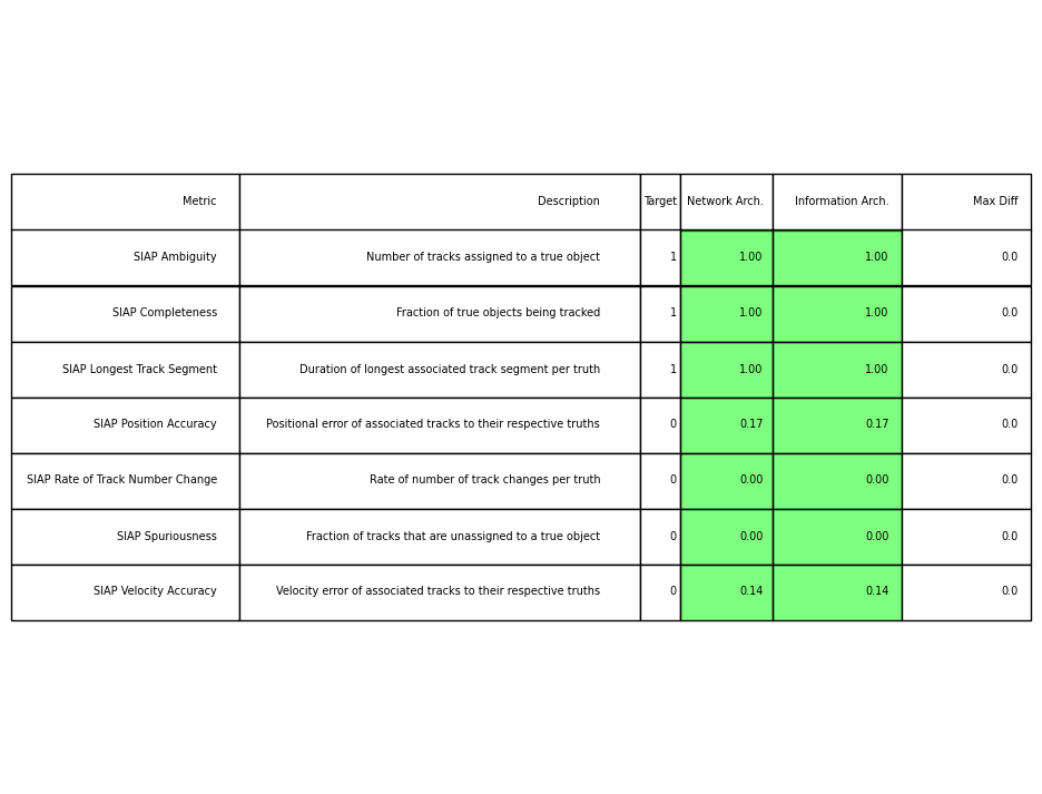
<matplotlib.table.Table object at 0x6ffea53bc260>

5 - Remove edges from each architecture and re-run

In this section, we take an identical copy of each of the architectures above, and remove an edge. We aim to show the following:

• It is possible to remove certain edges from a network architecture without affecting the performance of the network.

• Removing an edge from an information architecture will likely have an effect on performance.

First, we must set up the two architectures, and remove an edge from each. In the network architecture, there are multiple routes between some pairs of nodes. This redundency increases the resilience of the network when an edge, or node, is taken out of action. In this example, we remove edges connecting repeater node r3, in turn, disabling a route from sensor node s0 to fusion node f0. As another route from s0 to f0 exists (via repeater node r4), the performance of the network should not be effected (assuming unlimited bandwidth).

Network and Information arch pair

network_arch_rm = id_net_archs[2]
information_arch_rm = id_net_archs[3].information_arch

rm = []
for edge in network_arch_rm.edges:
    if 'r3' in [node.label for node in edge.nodes]:
        rm.append(edge)

for edge in rm:
    network_arch_rm.edges.remove(edge)

network_arch_rm

Now we remove an edge from the information architecture. You could choose pretty much any edge here, but removing the edge between sf0 and f1 is likely to cause the greatest destruction (in the interest of the reader). Removing this edge creates a disconnected graph. The Stone Soup architecture module can deal with this with no issues, but for this example we will now only consider the connected subgraph containing node f1.

rm = []
for edge in information_arch_rm.edges:
    if ('sf0' in [node.label for node in edge.nodes]) and \
     ('f1' in [node.label for node in edge.nodes]):
        rm.append(edge)

for edge in rm:
    information_arch_rm.edges.remove(edge)

information_arch_rm

We now run the simulation for both architectures and calculate the same SIAP metrics as we did before for the original architectures.

for time in timesteps:
    network_arch_rm.measure(truths, noise=True)
    network_arch_rm.propagate(time_increment=1)
    information_arch_rm.measure(truths, noise=True)
    information_arch_rm.propagate(time_increment=1)

top_node = [node for node in network_arch_rm.all_nodes if node.label == 'f1'][0]

network_rm_siap = SIAPMetrics(position_measure=Euclidean((0, 2)),
                              velocity_measure=Euclidean((1, 3)),
                              generator_name='network_rm_siap',
                              tracks_key='network_rm_tracks',
                              truths_key='truths'
                              )

network_rm_metric_manager = MultiManager([network_rm_siap], associator)
network_rm_metric_manager.add_data({'network_rm_tracks': top_node.tracks,
                                    'truths': truths}, overwrite=False)
network_rm_metrics = network_rm_metric_manager.generate_metrics()

network_rm_siap_metrics = network_rm_metrics['network_rm_siap']
network_rm_siap_averages = {network_rm_siap_metrics.get(metric) for
                            metric in network_rm_siap_metrics
                            if metric.startswith("SIAP") and not metric.endswith(" at times")}

top_node = [node for node in information_arch_rm.all_nodes if node.label == 'f1'][0]

information_rm_siap = SIAPMetrics(position_measure=Euclidean((0, 2)),
                                  velocity_measure=Euclidean((1, 3)),
                                  generator_name='information_rm_siap',
                                  tracks_key='information_rm_tracks',
                                  truths_key='truths'
                                  )

information_rm_metric_manager = MultiManager([information_rm_siap],
                                             associator)  # associator for generating SIAP metrics
information_rm_metric_manager.add_data({'information_rm_tracks': top_node.tracks,
                                        'truths': truths}, overwrite=False)
information_rm_metrics = information_rm_metric_manager.generate_metrics()

information_rm_siap_metrics = information_rm_metrics['information_rm_siap']
information_rm_siap_averages = {information_rm_siap_metrics.get(metric) for
                                metric in information_rm_siap_metrics
                                if metric.startswith("SIAP") and not metric.endswith(" at times")}

Plotting the metrics for the two original architectures, and the metrics for the copies with edges removed, should display the result we predicted at the start of this section.

SIAPDiffTableGenerator([network_siap_averages,
                        information_siap_averages,
                        network_rm_siap_averages,
                        information_rm_siap_averages],
                       ['Network', 'Info', 'Network RM', 'Info RM'],
                       rtol=1e-2, atol=1e-5).compute_metric()

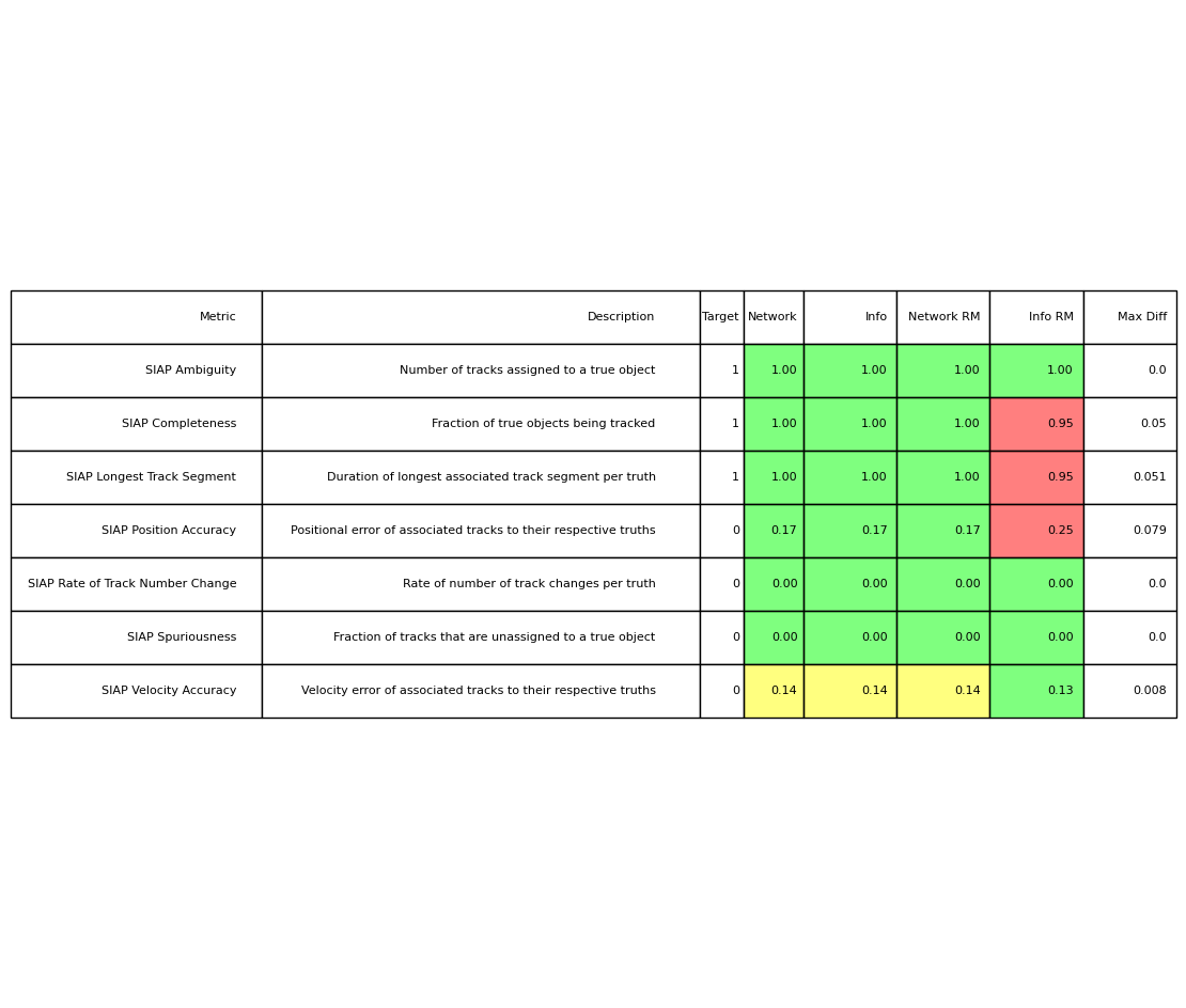
<matplotlib.table.Table object at 0x6ffe863891c0>