Note
Go to the end to download the full example code or to run this example in your browser via Binder.
\(k\)-d trees and TPR trees
\(k\)-d trees and TPR trees are both data structures which can be used to index objects in multi-dimensional space.
A \(k\)-d tree is useful for indexing the positions of static objects. It can be used to index \(k\)-dimensional data, where \(k\) represents any number of dimensions.
A \(k\)-d tree can also be used to index the positions of moving objects, but it will only show a snapshot of positions at a given time step so must be reconstructed at each time step.
A TPR tree (time-parameterised range tree) can be used to store and query information about moving objects. The tree stores functions of time that use the position and velocity of an object at a given time point to return the current or predicted future positions of the object.
A TPR tree does not need to be reconstructed at every time step which saves computing power, but it should be occasionally updated with new position and velocity information to maintain accuracy. The frequency of updates depends on the desired accuracy and the movement exhibited by objects stored in the tree. E.g. frequent changes in the velocity or direction of an object would require more frequent tree updates to maintain higher accuracy.
Using \(k\)-d trees or TPR trees for data association
During Nearest Neighbour or Probabilistic Data Association without a tree, distance or probability of association must be calculated between the prediction and every detection in order to select the best detection for association. These linear searches can be a suitable method to use for small numbers of detections and/or targets but become inefficient if the numbers increase substantially.
Using a tree in combination with a data association algorithm can make the search much faster. Instead of comparing every detection in the set to the prediction vector, \(k\)-d trees or TPR trees can be used to quickly eliminate large sets of detections implicitly. Given a set of \(n\) detections, \(k\)-d trees have an average search time of O(\(log(n)\)) and a worst case of O(\(n\)).
We will look at how \(k\)-d trees are constructed and queried below.
Constructing a \(k\)-d tree
\(k\)-d trees are constructed by splitting a set of detections into two even groups, and then further splitting each of those two groups in half again, continuing this process recursively downwards until each leaf node contains the desired number of detections (it can be 1 or more). These splits alternate in each dimension of the detection vectors in turn until they reach the \(k^{th}\) dimension, at which point the splitting continues from the first dimension again (Fig. 1).
For example, with a set of 2-dimensional detection vectors of \(\small\begin{bmatrix} x \\ y \\\end{bmatrix}\) we start constructing the tree from the root node by identifying the median value of the \(x^{th}\) dimension of all detections. The detection with median value becomes the root node.
All detections with \(x\) coordinate \(\leq\) the median are placed in the left subtree from the root node, and all detections with \(x\) coordinate \(>\) median are placed in the right subtree from the root node. The left and right subtrees are then split into two further subtrees in the same way, except this time using the values in the \(y^{th}\) dimension in place of the \(x^{th}\). The third split is done in the \(x^{th}\) dimension again and so on until you achieve a determined number of points in each leaf node. Using a split at the median is just one common way to construct it.
Generation of a \(k\)-d tree has O(\(nlog^2n\)) time.
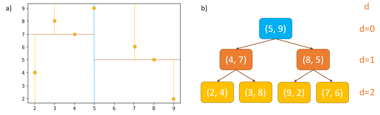
Fig. 1 shows the construction of a \(k\)-d tree. \(d\) represents the depth of the tree. At \(d=0\) the split occurs in the \(x\)-axis, at \(d=1\) the split occurs in the \(y\)-axis etc.
In comparison, entries in TPR tree leaf nodes are pairs of a moving object’s position and its ID. The internal nodes of the tree are bounding rectangles which bound the positions of all moving objects (or other bounding rectangles) in that subtree. The bounding rectangles’ coordinates are functions of time, so they are capable of following the enclosed object positions as they move over time.
Searching a \(k\)-d tree with Nearest Neighbour
The method for searching the tree is similar to the method for building the tree: starting at the root node, the \(x^{th}\) dimension of the prediction vector is compared with the \(x^{th}\) dimension of the root node detection vector. If the value of the prediction’s \(x\) dimension is less than or equal to that of the root node detection, the search moves down the left subtree, and down the right subtree if the value is greater. This process is repeated recursively at each internal node, again alternating through the vector dimensions, until a leaf node is reached. See Figure 2 for example.
To find the nearest neighbour to the prediction, at each node the Euclidean distance between the prediction and the detection at that node is measured. If the distance is less than the current best distance, the detection at that node becomes the new current best nearest neighbour.
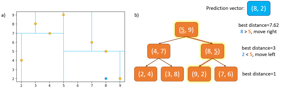
Fig. 2a shows the detections (orange) and the prediction vector, \([8,2]\) (blue). 2b shows the search down the \(k\)-d tree with current best distance shown on the right side. We start at the root node detection, where distance from prediction = 7.62 units. We look at the \(x^{th}\) dimension of the prediction \([8,2]\) and detection \([5,9]\) vectors. 8 > 5 so we move right down the tree to detection \([8,5]\) where distance from prediction = 3. Now we look at the \(y^{th}\) dimension of the vectors: 2 < 5 so we move left to the leaf node containing detection \([9,2]\) where distance from prediction = 1. The search then continues back up the tree and as there are no sibling subtrees that can beat the current best, the detection at \([9,2]\) is selected as the nearest neighbour.
Once we reach a leaf node the search must continue back up through the tree to ensure we haven’t missed a potential nearest neighbour that lies in an unexplored subtree. An unexplored subtree will only be searched if it could possibly contain a closer detection than the current nearest neighbour.
Looking at Figure 3 for example, after traversing completely down the tree, our current nearest neighbour to our prediction vector \([9,6]\) is detection \([7,5]\) with a distance of 2.24 units. Figure 3a shows that the shortest distance between the prediction (blue) and unexplored subtree (shaded area) is 1 unit (shown by red arrow).
This means that there could be a detection in the unexplored subtree with a distance from prediction of between 1 and 2.24 units, i.e. less than our current best of 2.24. So, we search down the left subtree from detection \([7,5]\). Indeed, there is a detection at \([9,4]\) in this subtree which has a distance from our prediction vector of 2 units, which becomes the new best distance. We then traverse back up the tree again. There are no other subtrees in the tree which can possibly contain detections that beat the current best distance, so the detection at \([9,4]\) is selected as the nearest neighbour and the search is complete when we reach the root.
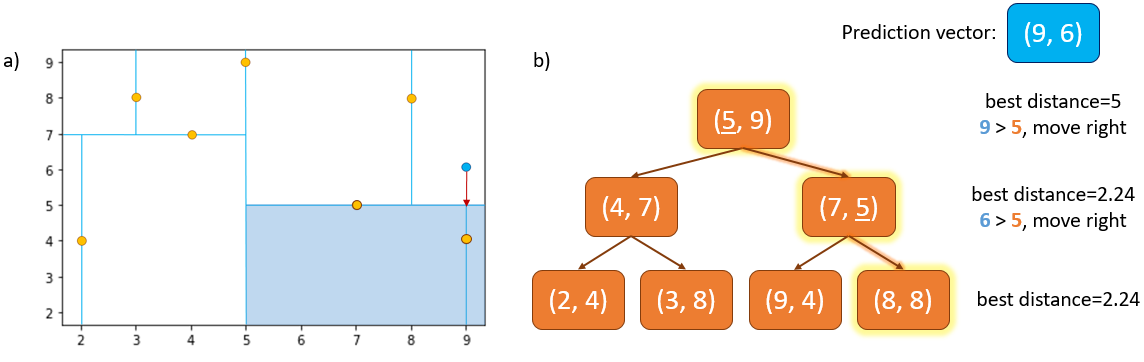
Fig. 3 shows a situation where it is useful to traverse back up the tree to complete the search for the nearest neighbour. The detection \([9,4]\) is the true nearest neighbour.
\(k\)-d and TPR trees can both be searched with Nearest Neighbour or Probabilistic Data Association algorithms. Using the tree will increase the efficiency of searches where there are more targets and/or detections.
Example of Global Nearest Neighbour search using \(k\)-d tree and TPR tree
In this example, we will be calculating the average run time of the Global Nearest Neighbour (GNN) data association algorithm with a \(k\)-d tree and with a TPR tree and comparing the results with a linear GNN search. First, we will run the search with a \(k\)-d tree.
Simulate ground truth
We will simulate a large number of targets moving in the \(x\), \(y\) Cartesian plane. We will then add detections with a high clutter rate at each time step.
import datetime
from itertools import tee

import numpy as np

from stonesoup.types.array import StateVector, CovarianceMatrix
from stonesoup.types.state import GaussianState

initial_state_mean = StateVector([[0], [0], [0], [0]])
initial_state_covariance = CovarianceMatrix(np.diag([4, 0.5, 4, 0.5]))
timestep_size = datetime.timedelta(seconds=5)
number_of_steps = 25
birth_rate = 0.3
death_probability = 0.05
initial_state = GaussianState(initial_state_mean, initial_state_covariance)

from stonesoup.models.transition.linear import (
    CombinedLinearGaussianTransitionModel, ConstantVelocity)

transition_model = CombinedLinearGaussianTransitionModel(
    [ConstantVelocity(0.05), ConstantVelocity(0.05)])

from stonesoup.simulator.simple import MultiTargetGroundTruthSimulator

groundtruth_sims = [
    MultiTargetGroundTruthSimulator(
        transition_model=transition_model,
        initial_state=initial_state,
        timestep=timestep_size,
        number_steps=number_of_steps,
        birth_rate=birth_rate,
        death_probability=death_probability,
        initial_number_targets=100)
    for _ in range(3)]
Initialise the measurement models
from stonesoup.simulator.simple import SimpleDetectionSimulator
from stonesoup.models.measurement.linear import LinearGaussian

# initialise the measurement model
measurement_model_covariance = np.diag([0.25, 0.25])
measurement_model = LinearGaussian(4, [0, 2], measurement_model_covariance)

# probability of detection
probability_detection = 0.9

# clutter will be generated uniformly in this are around the target
clutter_area = np.array([[-1, 1], [-1, 1]]) * 500
clutter_rate = 50

detection_sims = [
   SimpleDetectionSimulator(
        groundtruth=groundtruth_sim,
        measurement_model=measurement_model,
        detection_probability=probability_detection,
        meas_range=clutter_area,
        clutter_rate=clutter_rate)
   for groundtruth_sim in groundtruth_sims]

# Use tee to create 3 identical versions, for GNN, k-D tree and TPR-Tree
sim_sets = [tee(sim, 3) for sim in detection_sims]
sim_sets = list(zip(*sim_sets))
Import tracker components
# tracker predictor and updater
from stonesoup.predictor.kalman import KalmanPredictor
from stonesoup.updater.kalman import KalmanUpdater

# initiator and deleter
from stonesoup.deleter.error import CovarianceBasedDeleter
from stonesoup.initiator.simple import MultiMeasurementInitiator

# tracker
from stonesoup.tracker.simple import MultiTargetTracker

# timer for comparing run time of k-d tree algorithm with linear search
import time as timer
1. Run the search with a \(k\)-d tree
Set up the \(k\)-d tree to operate with the GNN algorithm to identify the most likely nearest neighbours to each track globally.
# create predictor and updater
predictor = KalmanPredictor(transition_model)
updater = KalmanUpdater(measurement_model)

# create hypothesiser
from stonesoup.hypothesiser.distance import DistanceHypothesiser
from stonesoup.measures import Mahalanobis

hypothesiser = DistanceHypothesiser(predictor, updater, measure=Mahalanobis(), missed_distance=3)

# create KD-tree data associator
from stonesoup.dataassociator.tree import DetectionKDTreeGNN2D

KD_data_associator = DetectionKDTreeGNN2D(hypothesiser=hypothesiser,
                                          predictor=predictor,
                                          updater=updater,
                                          number_of_neighbours=3,
                                          max_distance_covariance_multiplier=3)
Create tracker and run it
run_times_KDTree = []

# run loop to calculate average run time
for n, detection_sim in enumerate(sim_sets[0]):
    start_time = timer.perf_counter()

    # create tracker components
    predictor = KalmanPredictor(transition_model)
    updater = KalmanUpdater(measurement_model)

    # create deleter
    covariance_limit_for_delete = 100
    deleter = CovarianceBasedDeleter(covar_trace_thresh=covariance_limit_for_delete)

    # create initiator
    s_prior_state = GaussianState([[0], [0], [0], [0]], np.diag([0, 0.5, 0, 0.5]))
    min_detections = 3

    initiator = MultiMeasurementInitiator(
        prior_state=s_prior_state,
        measurement_model=measurement_model,
        deleter=deleter,
        data_associator=KD_data_associator,
        updater=updater,
        min_points=min_detections
    )

    # create tracker
    tracker = MultiTargetTracker(
        initiator=initiator,
        deleter=deleter,
        detector=detection_sim,
        data_associator=KD_data_associator,
        updater=updater
    )

    # run tracker
    groundtruth = set()
    detections = set()
    tracks = set()

    for time, ctracks in tracker:
        groundtruth.update(groundtruth_sims[n].groundtruth_paths)
        detections.update(detection_sims[n].detections)
        tracks.update(ctracks)

    end_time = timer.perf_counter()
    run_time = end_time - start_time

    run_times_KDTree.append(run_time)
Plot the resulting tracks from \(k\)-d tree
from stonesoup.plotter import Plotterly

plotter = Plotterly()
plotter.plot_ground_truths(groundtruth, mapping=[0, 2])
plotter.plot_measurements(detections, mapping=[0, 2])
plotter.plot_tracks(tracks, mapping=[0, 2])
plotter.fig
2. Run the search with a TPR tree
Now we will construct a TPR tree to operate with the same GNN algorithm to identify the most likely nearest neighbours to each track globally to compare run times.
# create the TPR tree data associator
from stonesoup.dataassociator.tree import TPRTreeGNN2D

TPR_data_associator = TPRTreeGNN2D(hypothesiser=hypothesiser,
                                   measurement_model=measurement_model,
                                   horizon_time=datetime.timedelta(seconds=10))

run_times_TPRTree = []

for detection_sim in sim_sets[1]:
    start_time = timer.perf_counter()

    TPR_data_associator = TPRTreeGNN2D(hypothesiser=hypothesiser,
                                       measurement_model=measurement_model,
                                       horizon_time=datetime.timedelta(seconds=10))

    # create predictor and updater
    predictor = KalmanPredictor(transition_model)
    updater = KalmanUpdater(measurement_model)

    # create deleter
    covariance_limit_for_delete = 100
    deleter = CovarianceBasedDeleter(covar_trace_thresh=covariance_limit_for_delete)

    # create initiator
    s_prior_state = GaussianState([[0], [0], [0], [0]], np.diag([0, 0.5, 0, 0.5]))
    min_detections = 3

    initiator = MultiMeasurementInitiator(
        prior_state=s_prior_state,
        measurement_model=measurement_model,
        deleter=deleter,
        data_associator=TPR_data_associator,
        updater=updater,
        min_points=min_detections
    )

    # create tracker
    tracker = MultiTargetTracker(
        initiator=initiator,
        deleter=deleter,
        detector=detection_sim,
        data_associator=TPR_data_associator,
        updater=updater
    )

    # run tracker
    tracks = set()

    for time, ctracks in tracker:
        tracks.update(ctracks)

    end_time = timer.perf_counter()
    run_time = end_time - start_time

    run_times_TPRTree.append(run_time)
Plot the resulting tracks from TPR Tree
from stonesoup.plotter import Plotterly

plotter = Plotterly()
plotter.plot_ground_truths(groundtruth, mapping=[0, 2])
plotter.plot_measurements(detections, mapping=[0, 2])
plotter.plot_tracks(tracks, mapping=[0, 2])
plotter.fig
3. Run the search with a linear search
Now, to compare computing time, we will run a linear Global Nearest Neighbour search.
# set up GNN data associator
from stonesoup.dataassociator.neighbour import GNNWith2DAssignment
GNN_data_associator = GNNWith2DAssignment(hypothesiser=hypothesiser)

run_times_GNN = []

# run loop to calculate average run time
for detection_sim in sim_sets[2]:
    start_time = timer.perf_counter()

    # create tracker components
    predictor = KalmanPredictor(transition_model)
    updater = KalmanUpdater(measurement_model)

    # create deleter
    covariance_limit_for_delete = 100
    deleter = CovarianceBasedDeleter(covar_trace_thresh=covariance_limit_for_delete)

    s_prior_state = GaussianState([[0], [0], [0], [0]], np.diag([0, 0.5, 0, 0.5]))
    min_detections = 3

    # create initiator
    initiator = MultiMeasurementInitiator(
        prior_state=s_prior_state,
        measurement_model=measurement_model,
        deleter=deleter,
        data_associator=GNN_data_associator,
        updater=updater,
        min_points=min_detections
    )

    # create tracker
    tracker = MultiTargetTracker(
        initiator=initiator,
        deleter=deleter,
        detector=detection_sim,
        data_associator=GNN_data_associator,
        updater=updater
    )

    # run tracker
    tracks = set()

    for time, ctracks in tracker:
        tracks.update(ctracks)

    end_time = timer.perf_counter()
    run_time = end_time - start_time

    run_times_GNN.append(run_time)
Plot the resulting tracks from GNN
from stonesoup.plotter import Plotterly

plotter = Plotterly()
plotter.plot_ground_truths(groundtruth, mapping=[0, 2])
plotter.plot_measurements(detections, mapping=[0, 2])
plotter.plot_tracks(tracks, mapping=[0, 2])
plotter.fig
Compare search times
from statistics import median

print(f'Median run time of k-d tree search: {round(median(run_times_KDTree), 4)} seconds')
print(f'Median run time of TPR tree search: {round(median(run_times_TPRTree), 4)} seconds')
print(f'Median run time of linear search: {round(median(run_times_GNN), 4)} seconds')
print(f'\nThe GNN search runs {round(median(run_times_GNN)/median(run_times_KDTree), 2)} times faster on average with '
      f'kd-tree than with linear search')
print(f'\nThe GNN search runs {round(median(run_times_GNN)/median(run_times_TPRTree), 2)} times faster on average with '
      f'TPR tree than with linear search')
Median run time of k-d tree search: 4.8345 seconds
Median run time of TPR tree search: 4.6048 seconds
Median run time of linear search: 11.7129 seconds

The GNN search runs 2.42 times faster on average with kd-tree than with linear search

The GNN search runs 2.54 times faster on average with TPR tree than with linear search
In the tracking situation chosen for this example, where we have 200 targets and relatively high probability of detection (90%), the \(k\)-d tree outperforms the TPR tree, and both outperform the linear search in terms of computing time. The TPR tree can outperform the \(k\)-d tree in tracking situations with a significantly higher number of targets and a lower probability of detection.
You can change these parameters in the code above and see how the run times of the GNN algorithm are affected by the different data indexing structures demonstrated.
Total running time of the script: (1 minutes 12.305 seconds)