Particle Filter Resamplers: Tutorial

import numpy as np

Introduction

Stone Soup comes with a number of resamplers, for the Particle Filter, that can be used straight out of the box. This example explains each of the resamplers and compares the results of using each one.

Resamplers currently available in Stone Soup:

• SystematicResampler

• MultinomialResampler

• StratifiedResampler

• ResidualResampler

• ESSResampler (Effective Sample Size Resampler)

The last two resamplers (Residual and ESS) are preprocessing methods that require the use of another resampler.

Plotter for this notebook

import matplotlib.pyplot as plt


def plot(normalised_weights, u_j=None, stratified=False, residual=False):
    nparts = len(normalised_weights)
    floors = np.floor(normalised_weights * nparts)

    # Plot
    fig, ax = plt.subplots()
    fig.set_size_inches(10, 1.5)
    plt.xlim([0, 1])
    for i, particle_weight in enumerate(normalised_weights):
        l = 0
        for j in range(i):
            l += normalised_weights[j]
        ax.barh(['CDF'], [particle_weight], left=l)
        if residual is not False:
            if floors[i] != 0:
                ax.barh(['CDF'], [(1 / nparts) * floors[i]], left=l, color='White')

    if u_j is not None:
        plt.plot([u_j, u_j], [-0.4, 0.4], 'k-', lw=4)
    if stratified is not False:
        plt.plot([s_lb, s_lb], [-0.4, 0.4], 'w:', lw=2)

Cumulative Distribution Function

The Systematic, Multinomial, and Stratified resamplers all use a cumulative distribution function (CDF) to randomly pick points from. The CDF is calculated from the cumulative sum of the normalised weights of the existing particles.

Example

Given the following set of particles and their weights:

Particle Weights

Particle	Weight	Normalised Weight
1	1	0.1
2	5	0.5
3	1.5	0.15
4	0.5	0.05
5	2	0.2

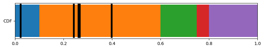
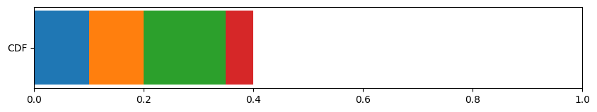
We would calculate the following CDF:

particle_weights = [1, 5, 1.5, 0.5, 2]
n_particles = len(particle_weights)

normalised_weights = np.array([particle/sum(particle_weights) for particle in particle_weights])
plot(normalised_weights)

Each of the resamplers then use a different method to pick points in the CDF. For example, assume the following points are picked: 0.15, 0.41, 0.57, 0.63, and 0.89. These points are shown on the CDF below.

u_j = [0.15, 0.41, 0.57, 0.63, 0.89]
plot(normalised_weights, u_j)

As shown above, the points 0.15, 0.41, and 0.57 all fall within the section of the CDF corresponding to particle 2, while the points 0.63 and 0.89 fall within the sections of the CDF corresponding to particles 3 and 5, respectively.

Hence, for this example, the number of times each particle is resampled is as follows:

Particle Weights

Particle	No. of times resampled	Weight of new resampled particles
1	0	0.2
2	3	0.2
3	1	0.2
4	0	0.2
5	1	0.2

As shown in the table, the resampler assigns a new weight to each sample - by default, each of the resamplers included in Stone Soup give all particles an equal weight of \(1/N\) where \(N\) = no. of resampled particles.

Resamplers

Multinomial Resampler

The MultinomialResampler calculates \(N\) independent random numbers from the uniform distribution \(u \sim U(0,1]\), where \(N\) is the target number of particles to be resampled. In most cases, we use \(N = M\), where \(M\) is the number of existing particles to be resampled. However, the Multinomial resampler can upsample (\(N > M\)) or downsample (\(N < M\)) to a value \(N \neq M \in \mathbb{N}\). The Multinomial resampler has a computational complexity of \(O(MN)\) where \(N\) and \(M\) are the number of resampled and existing particles respectively.

An example of how the Multinomial resampler picks points from the CDF is shown below. Black lines represent the chosen points.

import numpy as np

# Pick N random points in the uniform distribution u~U(0,1]
u_j = np.random.rand(5)

plot(normalised_weights, u_j)

Systematic Resampler

Unlike the Multinomial resampler, the SystematicResampler doesn’t calculate all points independently. Instead, a single random starting point in the range \([0,1/N]\) is chosen. \(N\) points are then calculated at equidistant intervals along the CDF, so that there is a gap of \(1/N\) between any two consecutive points. The Systematic resampler has a computational complexity of \(O(N)\) where \(N\) is the number of resampled particles.

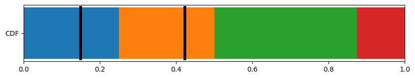
An example of how the Systematic resampler picks points from the CDF is shown below. Black lines represent the chosen points.

# Pick a starting point
s = np.random.uniform(0, 1/n_particles)

# Calculate N equidistant points from the starting point
u_j = s + (1 / n_particles) * np.arange(n_particles)

plot(normalised_weights, u_j)

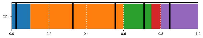
Stratified Resampler

The StratifiedResampler splits the whole CDF into \(N\) evenly sized strata (subpopulations). A random point is then chosen, independently, from each stratum. This results in the gap between any two consecutive points being in the range \((0, 2/N]\). The Stratified resampler has a computational complexity of \(O(N)\) where \(N\) is the number of resampled particles.

An example of how the Stratified resampler picks points from the CDF is shown below. Black lines represent the chosen points, with white dashed lines representing the strata boundaries.

# Calculate lower bound of each stratum
s_lb = np.arange(n_particles) * (1 / n_particles)

# Independently pick a point from each stratum
u_j = np.random.uniform(s_lb, s_lb + (1 / n_particles))

plot(normalised_weights, u_j, s_lb)

Preprocessing methods

Residual Resampler

The ResidualResampler consists of two stages.

Stage 1

The first stage determines which particles have weight \(w^{i} \geq 1/N\), where \(i \in 1, ..., N\) denotes each particle. Each of these particles is then resampled \(N^{i}_{j} = floor(Nw^{i}_{j})\) times, where \(j \in 1, 2\) denotes the stage. Hence, \(N_1 = \sum_{i=1}^{N}N^i_1\) represents the number of particles that are sampled in stage 1. As these weights have been represented in the resampled set of particles, we are only interested in the residual weights, left after the floor weights (\(N^{i}_{1}\)) have been subtracted.

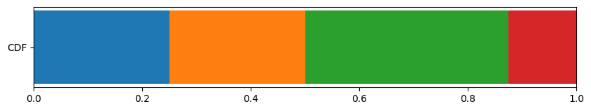
Reconsider our example with 5 particles, with weights shown by the plot below.

plot(normalised_weights)

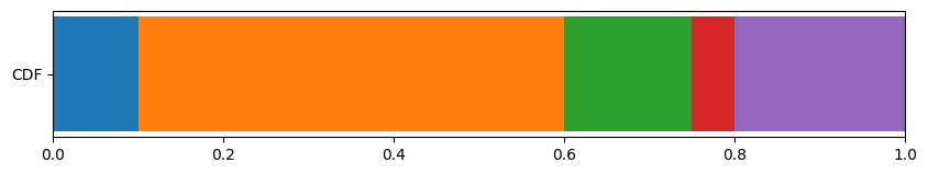
As we’re interested in particles of weight \(w^{i} \geq 1/N\), in this example we’re looking for particles with \(w^{i} \geq 1/5\). Hence Particle 2 (orange, weight = 0.5) and Particle 5 (purple, weight = 0.2). We resample these particles \(N^{i}_{j} = floor(Nw^{i}_{j})\) times:

• Particle 2 gets resampled \(N^{2}_{1} = floor(Nw^{2}_{1}) = floor(5 * 0.5) = 2\) times.

• Particle 5 gets resampled \(N^{5}_{1} = floor(Nw^{5}_{1}) = floor(5 * 0.2) = 1\) times.

• Particles 1, 3 and 4 do not get resampled as their weights are \(\leq 1/5\).

A total of 3 particles were sampled from stage 1 (2x Particle 2, 1x Particle 5), hence \(N_1 = \sum_{i=1}^{N}N^i_1 = 3\)

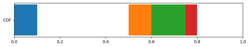
Original CDF with floor weights removed:

plot(normalised_weights, residual=True)

New CDF:

floors = np.floor(normalised_weights * n_particles)
residuals = (normalised_weights - floors/n_particles)
plot(residuals)

The CDF of the residual weights is carried on to stage 2.

Stage 2

We now look to resample the remaining \(N_2 = N - N_1\) particles during stage 2. (Reminder: N is the total number of particles we want to sample, while \(N_1\) is the number of particles we have already resampled from stage 1). The residual weights from each particle are carried over from stage 1. These residual weights are normalised, and used to calculate a CDF, which is shown below.

Normalised residual weight CDF:

normalised_residual_weights = residuals*(1/sum(residuals))
plot(normalised_residual_weights)

We then use either the MultinomialResampler, StratifiedResampler, or SystematicResampler to sample the remaining \(N_2\) particles using the CDF.

Continuing with our example, we want to resample the remaining \(N_2 = N - N_1 = 5 - 3 = 2\) particles in stage 2. Here we will choose to use the MultinomialResampler (we could also use StratifiedResampler or SystematicResampler) to sample the \(N_2 = 2\) particles from the normalised residual weight CDF - more detail on how this is done can be found in the Multinomial Resampler section above.

u_j = np.random.rand(2)

plot(normalised_residual_weights, u_j)

This method reduces the number of particles that are sampled through the more computationally expensive methods seen above. The Residual resampler also guarantees that any particle of weight greater than \(1/N\) will be represented in the set of resampled particles.

When using the Residual resampler in Stone Soup, the Resampler requires a property ‘residual_resampler’. This property defines which resampler method to use for resampling the residuals in stage 2. The variable must be a string value from the following: ‘multinomial’, ‘systematic’, ‘stratified’. If no residual_method variable is provided, the multinomial method will be used by default.

ESS Resampler

The ESSResampler (Effective Sample Size) is a wrapper around another resampler. It performs a check at each time step to determine whether it is necessary to resample the particles. Resampling is only performed at a given time step if a defined criterion is met. Kish’s ESS criterion is used, which states that:

\[ESS = \left(\sum_{i=1}^{N} (W_{n}^i)^2\right)^{-1}\]

is less than or equal to the threshold, a float which is set by default to \(\frac{N}{2}\).

Example in Stone Soup

Generate some particles

An example of resampling particles using the Stone Soup resamplers. We generate some particles using the Particle class. In this example, we give every particle an equal weight - each particle will have the same likelihood of being resampled. The resample function returns a ParticleState. The state_vector property of which contains a list of particles to be resampled.

from stonesoup.types.particle import Particle

particles = [Particle(np.array([[i]]), weight=1/5) for i in range(5)]

Simple Example

In this example, we use the MultinomialResampler to resample the particles generated above. We simply define the Resampler and call its resample method.

There are situations where we may want to resample to a different number of particles - for example if you want more granular information, or want to be more computationally efficient. Excluding the ResidualResampler, all Stone Soup resamplers can up- or down-sample as shown below.

from stonesoup.resampler.particle import MultinomialResampler

# Resampler
resampler = MultinomialResampler()

# Resample particles
resampled_particles = resampler.resample(particles)
print("---- State vector of resampled particles ----")
print(resampled_particles.state_vector)
print("------ Weights of resampled particles -------")
print(resampled_particles.weight)

# Repeat while upsampling particles
upsampled_particles = resampler.resample(particles, nparts=10)
print("---- State vector of upsampled particles ----")
print(upsampled_particles.state_vector)
print("------ Weights of upsampled particles -------")
print(upsampled_particles.weight)

---- State vector of resampled particles ----
[[0 4 1 1 4]]
------ Weights of resampled particles -------
[Probability(0.2) Probability(0.2) Probability(0.2) Probability(0.2)
 Probability(0.2)]
---- State vector of upsampled particles ----
[[4 3 2 3 1 0 4 1 2 3]]
------ Weights of upsampled particles -------
[Probability(0.10000000000000002) Probability(0.10000000000000002)
 Probability(0.10000000000000002) Probability(0.10000000000000002)
 Probability(0.10000000000000002) Probability(0.10000000000000002)
 Probability(0.10000000000000002) Probability(0.10000000000000002)
 Probability(0.10000000000000002) Probability(0.10000000000000002)]

Here we can see which particles were chosen to be resampled and the weights of the new particles.

Example using ESS and ResidualResampler

In this example, we use both the Effecive Sample Size method, and the residual resampler, using the systematic method to resample the residuals.

from stonesoup.resampler.particle import ESSResampler, ResidualResampler

# Define Resampler
subresampler = ResidualResampler(residual_method='systematic')
resampler = ESSResampler(resampler=subresampler)

# Resample Particles
resampler.resample(particles)

ParticleState(
    state_vector=[[0 1 2 3 4]],
    timestamp=None,
    weight=array([Probability(0.2), Probability(0.2), Probability(0.2),
                  Probability(0.2), Probability(0.2)], dtype=object),
    log_weight=[-1.60943791 -1.60943791 -1.60943791 -1.60943791 -1.60943791],
    parent=None,
    particle_list=[Particle(
                      state_vector=[[0]],
                      weight=0.2,
                      parent=None),
                   Particle(
                      state_vector=[[1]],
                      weight=0.2,
                      parent=None),
                   Particle(
                      state_vector=[[2]],
                      weight=0.2,
                      parent=None),
                   Particle(
                      state_vector=[[3]],
                      weight=0.2,
                      parent=None),
                   Particle(
                      state_vector=[[4]],
                      weight=0.2,
                      parent=None)],
    fixed_covar=None)