3 - Optimised Sensor Management

This tutorial follows on from the Multiple Sensor Management tutorial and explores the use of external optimisation libraries to overcome the limitations of the brute force optimisation method introduced in the previous tutorial.

The scenario in this example is the same as Tutorial 2, simulating 3 targets moving on nearly constant velocity trajectories and an adjustable number of sensors. The sensors are RadarRotatingBearingRange with a defined field of view which can be pointed in a particular direction in order to make an observation.

The optimised sensor managers are built around SciPy’s ‘optimize’ library. Similar to the brute force method introduced previously, the sensor manager considers all possible configurations of sensors and actions and uses an optimising function with a specified reward function, returning the optimal configuration.

The UncertaintyRewardFunction is used for all sensor managers which chooses the configuration for which the sum of estimated uncertainties (as represented by the Frobenius norm of the covariance matrix) can be reduced the most by using the chosen sensing configuration.

As in the previous tutorials the SIAP [1] and uncertainty metrics are used to assess the performance of the sensor managers.

Sensor Management example

Setup

First, a simulation must be set up using components from Stone Soup. For this the following imports are required:

import numpy as np
import random
from ordered_set import OrderedSet
from datetime import datetime, timedelta

start_time = datetime.now().replace(microsecond=0)

from stonesoup.models.transition.linear import CombinedLinearGaussianTransitionModel, \
    ConstantVelocity
from stonesoup.types.groundtruth import GroundTruthPath, GroundTruthState

Generate ground truths

Generate transition model and ground truths as in Tutorials 1 & 2.

The number of targets in this simulation is defined by ntruths - here there are 3 targets travelling in different directions. The time the simulation is observed for is defined by time_max.

We can fix our random number generator to probe a particular example repeatedly. This can be undone by commenting out the first two lines in the next cell.

np.random.seed(1990)
random.seed(1990)

# Generate transition model
transition_model = CombinedLinearGaussianTransitionModel([ConstantVelocity(0.005),
                                                          ConstantVelocity(0.005)])

yps = range(0, 100, 10)  # y value for prior state
truths = OrderedSet()
ntruths = 3  # number of ground truths in simulation
time_max = 20  # timestamps the simulation is observed over
timesteps = [start_time + timedelta(seconds=k) for k in range(time_max)]

xdirection = 1
ydirection = 1

# Generate ground truths
for j in range(0, ntruths):
    truth = GroundTruthPath([GroundTruthState([0, xdirection, yps[j], ydirection],
                                              timestamp=timesteps[0])],
                            id=f"id{j}")

    for k in range(1, time_max):
        truth.append(
            GroundTruthState(transition_model.function(truth[k - 1], noise=True,
                                                       time_interval=timedelta(seconds=1)),
                             timestamp=timesteps[k]))
    truths.add(truth)

    xdirection *= -1
    if j % 2 == 0:
        ydirection *= -1

Plot the ground truths. This is done using the AnimatedPlotterly class from Stone Soup.

from stonesoup.plotter import AnimatedPlotterly

# Stonesoup plotter requires sets not lists

plotter = AnimatedPlotterly(timesteps, tail_length=1)
plotter.plot_ground_truths(truths, [0, 2])
plotter.fig

Create sensors

Create a set of sensors for each sensor management algorithm. As in Tutorial 2, this tutorial uses the RadarRotatingBearingRange sensor with the number of sensors initially set as 2 and each sensor positioned along the line \(x=10\), at distance intervals of 50.

n_sensors = 2

from stonesoup.types.state import StateVector
from stonesoup.sensor.radar.radar import RadarRotatingBearingRange
from stonesoup.types.angle import Angle

sensor_setA = set()
for n in range(0, n_sensors):
    sensor = RadarRotatingBearingRange(
        position_mapping=(0, 2),
        noise_covar=np.array([[np.radians(0.5) ** 2, 0],
                              [0, 1 ** 2]]),
        ndim_state=4,
        position=np.array([[10], [n * 50]]),
        rpm=60,
        fov_angle=np.radians(30),
        dwell_centre=StateVector([0.0]),
        max_range=np.inf,
        resolution=Angle(np.radians(30))
    )
    sensor_setA.add(sensor)
for sensor in sensor_setA:
    sensor.timestamp = start_time

sensor_setB = set()
for n in range(0, n_sensors):
    sensor = RadarRotatingBearingRange(
        position_mapping=(0, 2),
        noise_covar=np.array([[np.radians(0.5) ** 2, 0],
                              [0, 1 ** 2]]),
        ndim_state=4,
        position=np.array([[10], [n * 50]]),
        rpm=60,
        fov_angle=np.radians(30),
        dwell_centre=StateVector([0.0]),
        max_range=np.inf,
        resolution=Angle(np.radians(30))
    )
    sensor_setB.add(sensor)

for sensor in sensor_setB:
    sensor.timestamp = start_time

sensor_setC = set()
for n in range(0, n_sensors):
    sensor = RadarRotatingBearingRange(
        position_mapping=(0, 2),
        noise_covar=np.array([[np.radians(0.5) ** 2, 0],
                              [0, 1 ** 2]]),
        ndim_state=4,
        position=np.array([[10], [n * 50]]),
        rpm=60,
        fov_angle=np.radians(30),
        dwell_centre=StateVector([0.0]),
        max_range=np.inf,
        resolution=Angle(np.radians(30))
    )
    sensor_setC.add(sensor)

for sensor in sensor_setC:
    sensor.timestamp = start_time

Create the Kalman predictor and updater

Construct a predictor and updater using the KalmanPredictor and ExtendedKalmanUpdater components from Stone Soup. The measurement model for the updater is None as it is an attribute of the sensor.

from stonesoup.predictor.kalman import KalmanPredictor

predictor = KalmanPredictor(transition_model)

from stonesoup.updater.kalman import ExtendedKalmanUpdater

updater = ExtendedKalmanUpdater(measurement_model=None)
# measurement model is added to detections by the sensor

Run the Kalman filters

Create priors which estimate the targets’ initial states - these are the same as in the previous sensor management tutorials.

from stonesoup.types.state import GaussianState

priors = []
xdirection = 1.2
ydirection = 1.2
for j in range(0, ntruths):
    priors.append(GaussianState([[0], [xdirection], [yps[j] + 0.1], [ydirection]],
                                np.diag([0.5, 0.5, 0.5, 0.5] + np.random.normal(0, 5e-4, 4)),
                                timestamp=start_time))
    xdirection *= -1
    if j % 2 == 0:
        ydirection *= -1

Initialise the tracks by creating an empty list and appending the priors generated. This needs to be done separately for each sensor manager method as they will generate different sets of tracks.

from stonesoup.types.track import Track

# Initialise tracks from the BruteForceSensorManager
tracksA = {Track([prior]) for prior in priors}

# Initialise tracks from the OptimizeBruteSensorManager
tracksB = {Track([prior]) for prior in priors}

# Initialise tracks from the OptimizeBasinHoppingSensorManager
tracksC = {Track([prior]) for prior in priors}

Create sensor managers

The UncertaintyRewardFunction will be used for each sensor manager as in Tutorials 1 & 2 and the BruteForceSensorManager will be used as a comparison to the optimised methods.

from stonesoup.sensormanager.reward import UncertaintyRewardFunction
from stonesoup.sensormanager import BruteForceSensorManager

Optimised Brute Force Sensor Manager

The first optimised sensor manager, OptimizeBruteSensorManager, uses brute() which minimizes a function over a given range using a brute force method. This can be tailored by setting the number of grid points to search over or by adding the use of a polishing function.

from stonesoup.sensormanager import OptimizeBruteSensorManager

Optimised Basin Hopping Sensor Manager

The second optimised sensor manager, OptimizeBasinHoppingSensorManager, uses basinhopping() which finds the global minimum of a function using the basin-hopping algorithm. This is a combination of a global stepping algorithm and local minimization at each step. Parameters such as number of basin hopping iterations or step size can be set to tailor the algorithm to requirements.

from stonesoup.sensormanager import OptimizeBasinHoppingSensorManager

Initiate sensor managers

Create an instance of each sensor manager class. For the optimised sensor managers the default settings will be used meaning only a sensor set and reward function is required. The UncertaintyRewardFunction will be used for each sensor manager. For the OptimizeBruteSensorManager a polishing function is used by setting finish to True.

# initiate reward function
reward_function = UncertaintyRewardFunction(predictor, updater)

bruteforcesensormanager = BruteForceSensorManager(
    sensor_setA,
    reward_function=reward_function)

optimizebrutesensormanager = OptimizeBruteSensorManager(
    sensor_setB,
    reward_function=reward_function,
    finish=True)

optimizebasinhoppingsensormanager = OptimizeBasinHoppingSensorManager(
    sensor_setC,
    reward_function=reward_function)

Run the sensor managers

Each sensor management method requires a timestamp and a list of tracks at each time step when calling the function choose_actions(). This returns a mapping of sensors and actions to be taken by each sensor, decided by the sensor managers.

For each sensor management method, at each time step, the chosen action is given to the sensors and then measurements taken. The tracks are predicted and those with associated measurements are updated.

First, a hypothesiser and data associator are required for use in each tracker:

from stonesoup.hypothesiser.distance import DistanceHypothesiser
from stonesoup.measures import Mahalanobis
hypothesiser = DistanceHypothesiser(predictor, updater, measure=Mahalanobis(), missed_distance=5)

from stonesoup.dataassociator.neighbour import GNNWith2DAssignment
data_associator = GNNWith2DAssignment(hypothesiser)

Run brute force sensor manager

Each sensor manager is run in the same way as in the previous tutorials.

from ordered_set import OrderedSet
from collections import defaultdict
import time
import copy

# Start timer for cell execution time
cell_start_time1 = time.time()

sensor_history_A = defaultdict(dict)
for timestep in timesteps[1:]:

    # Generate chosen configuration
    chosen_actions = bruteforcesensormanager.choose_actions(tracksA, timestep)

    # Create empty dictionary for measurements
    measurementsA = set()

    for chosen_action in chosen_actions:
        for sensor, actions in chosen_action.items():
            sensor.add_actions(actions)

    for sensor in sensor_setA:
        sensor.act(timestep)
        sensor_history_A[timestep][sensor] = copy.copy(sensor)

        # Observe this ground truth
        measurementsA |= sensor.measure(OrderedSet(truth[timestep] for truth in truths),
                                        noise=True)

    hypotheses = data_associator.associate(tracksA,
                                           measurementsA,
                                           timestep)
    for track in tracksA:
        hypothesis = hypotheses[track]
        if hypothesis.measurement:
            post = updater.update(hypothesis)
            track.append(post)
        else:  # When data associator says no detections are good enough, we'll keep the prediction
            track.append(hypothesis.prediction)

cell_run_time1 = round(time.time() - cell_start_time1, 2)

Plot ground truths, tracks, and uncertainty ellipses for each target. The positions of the sensors are indicated by black x markers. This uses the Stone Soup AnimatedPlotterly plotter, with added code to plot the field of view of the sensor.

import plotly.graph_objects as go
from stonesoup.functions import pol2cart

plotterA = AnimatedPlotterly(timesteps, tail_length=1, sim_duration=10)
plotterA.plot_sensors(sensor_setA)
plotterA.plot_ground_truths(truths, [0, 2])
plotterA.plot_tracks(set(tracksA), [0, 2], uncertainty=True, plot_history=False)


def plot_sensor_fov(fig_, sensor_set, sensor_history):
    # Plot sensor field of view
    trace_base = len(fig_.data)
    for _ in sensor_set:
        fig_.add_trace(go.Scatter(mode='lines',
                                  line=go.scatter.Line(color='black',
                                                       dash='dash')))

    for frame in fig_.frames:
        traces_ = list(frame.traces)
        data_ = list(frame.data)

        timestring = frame.name
        timestamp = datetime.strptime(timestring, "%Y-%m-%d %H:%M:%S")

        for n_, sensor_ in enumerate(sensor_set):
            x = [0, 0]
            y = [0, 0]

            if timestamp in sensor_history:
                sensor_ = sensor_history[timestamp][sensor_]
                for i, fov_side in enumerate((-1, 1)):
                    range_ = min(getattr(sensor_, 'max_range', np.inf), 100)
                    x[i], y[i] = pol2cart(range_,
                                          sensor_.dwell_centre[0, 0]
                                          + sensor_.fov_angle / 2 * fov_side) \
                        + sensor_.position[[0, 1], 0]
            else:
                continue

            data_.append(go.Scatter(x=[x[0], sensor_.position[0], x[1]],
                                    y=[y[0], sensor_.position[1], y[1]],
                                    mode="lines",
                                    line=go.scatter.Line(color='black',
                                                         dash='dash'),
                                    showlegend=False))
            traces_.append(trace_base + n_)

        frame.traces = traces_
        frame.data = data_


plot_sensor_fov(plotterA.fig, sensor_setA, sensor_history_A)
plotterA.fig

The resulting plot is exactly the same as Tutorial 2.

Run optimised brute force sensor manager

# Start timer for cell execution time
cell_start_time2 = time.time()

sensor_history_B = defaultdict(dict)
for timestep in timesteps[1:]:

    # Generate chosen configuration
    chosen_actions = optimizebrutesensormanager.choose_actions(tracksB, timestep)

    # Create empty dictionary for measurements
    measurementsB = set()

    for chosen_action in chosen_actions:
        for sensor, actions in chosen_action.items():
            sensor.add_actions(actions)

    for sensor in sensor_setB:
        sensor.act(timestep)
        sensor_history_B[timestep][sensor] = copy.copy(sensor)

        # Observe this ground truth
        measurementsB |= sensor.measure(OrderedSet(truth[timestep] for truth in truths),
                                        noise=True)

    hypotheses = data_associator.associate(tracksB,
                                           measurementsB,
                                           timestep)
    for track in tracksB:
        hypothesis = hypotheses[track]
        if hypothesis.measurement:
            post = updater.update(hypothesis)
            track.append(post)
        else:  # When data associator says no detections are good enough, we'll keep the prediction
            track.append(hypothesis.prediction)

cell_run_time2 = round(time.time() - cell_start_time2, 2)

Plot ground truths, tracks and uncertainty ellipses for each target.

plotterB = AnimatedPlotterly(timesteps, tail_length=1, sim_duration=10)
plotterB.plot_sensors(sensor_setB)
plotterB.plot_ground_truths(truths, [0, 2])
plotterB.plot_tracks(tracksB, [0, 2], uncertainty=True, plot_history=False)
plot_sensor_fov(plotterB.fig, sensor_setB, sensor_history_B)
plotterB.fig

Run optimised basin hopping sensor manager

# Start timer for cell execution time
cell_start_time3 = time.time()

sensor_history_C = defaultdict(dict)
for timestep in timesteps[1:]:

    # Generate chosen configuration
    chosen_actions = optimizebasinhoppingsensormanager.choose_actions(tracksC, timestep)

    # Create empty dictionary for measurements
    measurementsC = set()

    for chosen_action in chosen_actions:
        for sensor, actions in chosen_action.items():
            sensor.add_actions(actions)

    for sensor in sensor_setC:
        sensor.act(timestep)
        sensor_history_C[timestep][sensor] = copy.copy(sensor)

        # Observe this ground truth
        measurementsC |= sensor.measure(OrderedSet(truth[timestep] for truth in truths),
                                        noise=True)

    hypotheses = data_associator.associate(tracksC,
                                           measurementsC,
                                           timestep)
    for track in tracksC:
        hypothesis = hypotheses[track]
        if hypothesis.measurement:
            post = updater.update(hypothesis)
            track.append(post)
        else:  # When data associator says no detections are good enough, we'll keep the prediction
            track.append(hypothesis.prediction)

cell_run_time3 = round(time.time() - cell_start_time3, 2)

Plot ground truths, tracks and uncertainty ellipses for each target.

plotterC = AnimatedPlotterly(timesteps, tail_length=1, sim_duration=10)
plotterC.plot_sensors(sensor_setC)
plotterC.plot_ground_truths(truths, [0, 2])
plotterC.plot_tracks(tracksC, [0, 2], uncertainty=True, plot_history=False)
plot_sensor_fov(plotterC.fig, sensor_setC, sensor_history_C)
plotterC.fig

At first glance, the plots for each of the optimised sensor managers show a very similar tracking performance to the BruteForceSensorManager.

Metrics

As in Tutorials 1 & 2 the SIAP and uncertainty metrics are used to compare the tracking performance of the sensor managers in more detail.

from stonesoup.metricgenerator.tracktotruthmetrics import SIAPMetrics
from stonesoup.measures import Euclidean

siap_generatorA = SIAPMetrics(position_measure=Euclidean((0, 2)),
                              velocity_measure=Euclidean((1, 3)),
                              generator_name='BruteForceSensorManager',
                              tracks_key='tracksA',
                              truths_key='truths')

siap_generatorB = SIAPMetrics(position_measure=Euclidean((0, 2)),
                              velocity_measure=Euclidean((1, 3)),
                              generator_name='OptimizeBruteSensorManager',
                              tracks_key='tracksB',
                              truths_key='truths')

siap_generatorC = SIAPMetrics(position_measure=Euclidean((0, 2)),
                              velocity_measure=Euclidean((1, 3)),
                              generator_name='OptimizeBasinHoppingSensorManager',
                              tracks_key='tracksC',
                              truths_key='truths')

from stonesoup.dataassociator.tracktotrack import TrackToTruth

associator = TrackToTruth(association_threshold=30)

from stonesoup.metricgenerator.uncertaintymetric import SumofCovarianceNormsMetric

uncertainty_generatorA = SumofCovarianceNormsMetric(generator_name="BruteForceSensorManager",
                                                    tracks_key="tracksA")

uncertainty_generatorB = SumofCovarianceNormsMetric(generator_name="OptimizeBruteSensorManager",
                                                    tracks_key="tracksB")

uncertainty_generatorC = SumofCovarianceNormsMetric(
    generator_name="OptimizeBasinHoppingSensorManager",
    tracks_key="tracksC")

Generate a metric manager.

from stonesoup.metricgenerator.manager import MultiManager

metric_manager = MultiManager([siap_generatorA,
                               siap_generatorB,
                               siap_generatorC,
                               uncertainty_generatorA,
                               uncertainty_generatorB,
                               uncertainty_generatorC],
                              associator=associator)

For each time step, data is added to the metric manager on truths and tracks. The metrics themselves can then be generated from the metric manager.

metric_manager.add_data({'truths': truths,
                         'tracksA': tracksA,
                         'tracksB': tracksB,
                         'tracksC': tracksC})

metrics = metric_manager.generate_metrics()

SIAP metrics

First we look at SIAP metrics. We are only interested in the positional accuracy (PA) and velocity accuracy (VA). These metrics can be plotted to show how they change over time.

from stonesoup.plotter import MetricPlotter

fig = MetricPlotter()
fig.plot_metrics(metrics, metric_names=['SIAP Position Accuracy at times',
                                        'SIAP Velocity Accuracy at times'],
                 color=['blue', 'orange', 'green'])

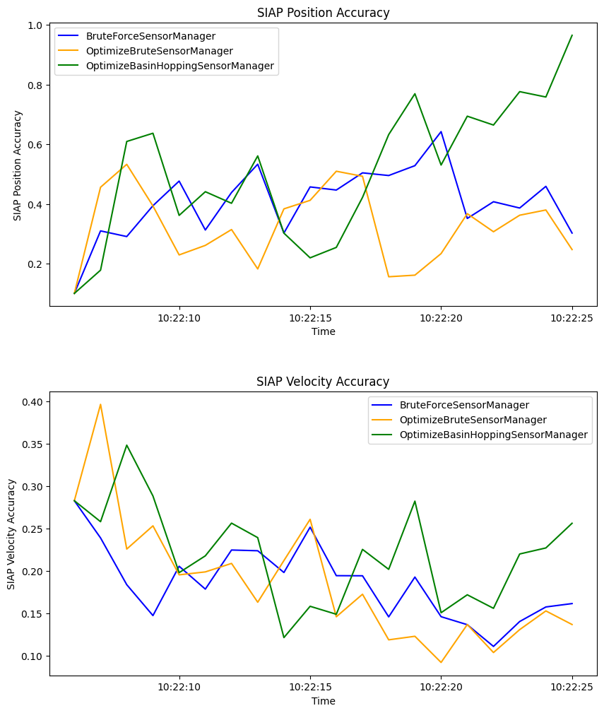
Both graphs show that there is little performance difference between the different sensor managers. Positional accuracy remains consistently good and velocity accuracy improves after overcoming the initial differences in the priors.

Uncertainty metric

Next, we look at the uncertainty metric which computes the sum of covariance matrix norms of each state at each time step. This is plotted over time for each sensor manager method.

fig2 = MetricPlotter()
fig2.plot_metrics(metrics, metric_names=['Sum of Covariance Norms Metric'],
                  color=['blue', 'orange', 'green'])

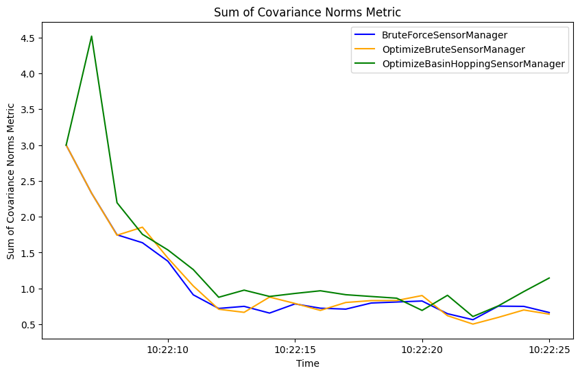
The uncertainty metric shows some variation between the sensor management methods, with a little more variation in the basin hopping method than the brute force methods. Overall they have a similar performance, improving after overcoming the initial differences in the priors.

Cell runtime

Now let us compare the calculated runtime of the tracking loop for each of the sensor managers.

import matplotlib.pyplot as plt

fig = plt.figure()
ax = fig.add_subplot(1, 1, 1)
ax.set_ylabel('Cell run time (s)')
ax.bar(['Brute Force', 'Optimised Brute Force', 'Optimised Basin Hopping'],
       [cell_run_time1, cell_run_time2, cell_run_time3],
       color=['tab:blue', 'tab:orange', 'tab:green'])

print(f'Brute Force: {cell_run_time1} s')
print(f'Optimised Brute Force: {cell_run_time2} s')
print(f'Optimised Basin Hopping: {cell_run_time3} s')

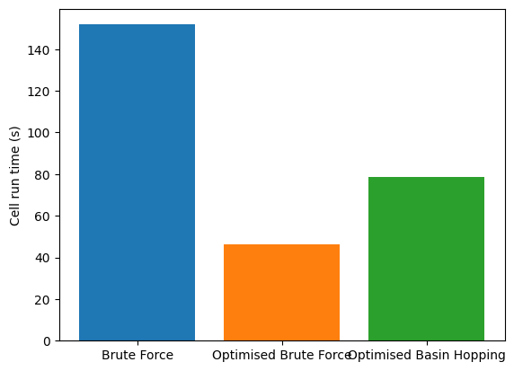
Brute Force: 53.66 s
Optimised Brute Force: 20.62 s
Optimised Basin Hopping: 34.88 s

The run times show that the optimised methods are significantly quicker than the brute force method whilst maintaining similar tracking performance. This difference becomes more clear when the complexity of the situation increases - by including additional sensors for example.

References

[1]

Votruba, Paul & Nisley, Rich & Rothrock, Ron and Zombro, Brett., Single Integrated Air Picture (SIAP) Metrics Implementation, 2001