Data Association with Loopy Belief Propagation

This example provides details of the Loopy Belief Propagation (LBP) algorithm [1] to perform data association in multiple target scenarios with measurement origin uncertainty. Through the utilisation of a graphical model formulation, we investigate how LBP can be leveraged to derive estimates of marginal association probabilities, which are crucial for establishing the correspondence between targets and measurements. Assuming that each target may generate at most one measurement, and each measurement is associated with at most one target, we focus on an approximate solution to a core problem in data association: calculating the marginal measurement-to-target association probabilities such as those used in the joint probabilistic data association (JPDA) filter [2]. In presence of multiple targets, we saw that the JPDA algorithm models the multi-target tracking problem, employing association variables to encode the relationship between targets and measurements. By introducing joint association events, encompassing all possible measurement-to-target assignment hypotheses, JPDA calculates the joint probability of each association event given the measurement set, subsequently updating target state estimates.

A critical aspect involves determining the marginal association probabilities \(p(a^i_{t}=j|Z_{1:t})\), indicating the likelihood that measurement \(j\) is associated with a target \(i\), with \(Z_{1:t}\) denoting the set of measurements up to time \(t\). Note that \(j=0\) denotes that no measurement is associated with target \(i\). These probabilities are derived by aggregating the joint probabilities over all events. However, exact calculation of these marginal probabilities, as in tutorial 8, entails exponential complexity in the number of targets/measurements, precluding the enumeration of all joint association events for large problem sizes. Herein lies the potential for LBP to offer a more computationally efficient (approximation) method, that offers scalability.

The graphical model formulation presented in [1] elucidates the association problem through a bipartite graph featuring target/measurement nodes interconnected by association variable links \(a^i_{t}\). BP operates on this graphical structure, facilitating message passing between neighbouring nodes to iteratively update beliefs/marginals pertaining to the association variables. Each iteration involves sending a message from each of the target association variables to each of the measurement association variables (and vice versa). Further elucidation on the graphical model employed is provided in the subsequent subsection.

Graphical model of the Belief Propagation

The graphical model formulation encapsulates the data association problem in multi-target tracking, aiming to efficiently represent and manipulate joint probability distributions of numerous variables through factorisation. Within this framework, Belief Propagation (BP) offers a streamlined approach to approximate the marginal probabilities \(p(a^i_{t}|Z_{1:t})\) without exhaustive enumeration. Optimal inference is facilitated on tree-structured graphs, where BP orchestrates message passing between nodes, iteratively refining beliefs/marginals based on received messages from neighbours.

A pivotal distinction lies in BP’s ability to approximate marginals without explicit enumeration and summation over all joint events, leveraging the factorisation of the joint distribution inherent in the graphical model. This strategy circumvents the exponential complexity associated with enumeration while retaining the capacity to capture multi-target interactions through the prescribed message passing regimen. Key components are as follows:

1. Graphical Model Formulation: The data association problem manifests as a bipartite graph, wherein targets and measurements are depicted as nodes. Association variables, denoted as \(a^i_{t}\) for each target \(i\), establish connections between target and measurement nodes. Specifically, \(a^i_{t}\) assumes a value measurement from 0 to \(M_t\), where \(M_t\) is the number of measurements at time \(t\), serving as an index from 1 to \(N_t\), where \(N_t\) is the number of targets at time \(t\).

2. Message Passing and Iterative Updates: LBP operates by exchanging messages among neighbouring nodes within the graph. Each message embodies the belief or marginal probability estimate from one node to another and is iteratively refined based on the product of received messages from neighbours, adhering to prescribed update rules derived from the graphical model factorisation. For instance, let \(\mu_{i\rightarrow j}\) denote the message from target node \(i\) to measurement node \(j\), and \(\nu_{j \rightarrow i}\) denote the message in the reverse direction.

   The updates follow:

\[\mu_{i\rightarrow j} = \frac{\psi_i(j)}{1+\sum_{j' \neq j, j'>0}\psi_i(j')\nu_{j' \rightarrow i}}\]

\[\nu_{j\rightarrow i} = \frac{1}{1+\sum_{i' \neq i, i'>0}\mu_{i' \rightarrow j}}\]

3. Belief Calculation: Upon convergence, LBP approximates the marginal as:

\[p(a^i_{t}=j|Z_{1:t}) \approx \frac{\psi_i(j) \nu_{j \rightarrow i}}{\sum_{j' } \psi_i(j' ) \nu_{j' \rightarrow i}}\]

The integration of BP within the JPDA framework offers the potential for significantly reduced computational complexity compared to exhaustive enumeration while still effectively capturing multi-target interactions. Unlike the enumeration, BP is scalable to complex scenarios (higher number of targets and measurements) and promises efficient approximation for the pivotal marginal calculation within the JPDA framework.

Exemplar of data association approach using enumeration and BP

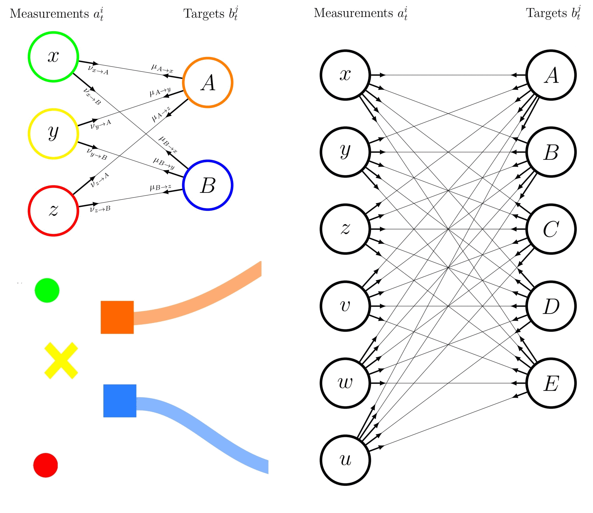
The following exemplifies the difference between an enumeration-based JPDA and the BP-based JPDA approach while estimating the marginal association probabilities in the context of 2 tracks (\(A\) and \(B\)) and 3 measurements (\(x\), \(y\), and \(z\), including a missed detection).

Using the enumeration-based JPDA, the marginal association probabilities \(p(a^i_{t}|Z_{1:t})\) represents the probability that measurement \(a^i_{t} = j\) is associated with track \(i\). The latter are computed by enumerating over all possible joint association events and summing the joint probabilities for events where the desired association occurs. Let’s denote the joint association events as \(a^i_t=j \in \left\{None, x, y, z\right\}\), where \(None\) refers to a false alarm detection, associate to the targets \(i \in \{A, B\}\). The marginal probability that measurement \(x\) is associated with track A, denoted as \(p(a^A_t=x | Z_{1:t})\), is calculated as:

\[\begin{split}p(a^A_t=x | Z_{1:t}) &= \bar{p}(a^A_t=x \cap a^B_t=None | Z_{1:t}) \\ &+ \bar{p}(a^A_t=x \cap a^B_t=y | Z_{1:t}) \\ &+ \bar{p}(a^A_t=x \cap a^B_t=z | Z_{1:t})\end{split}\]

where \(\bar{p}(\textit{multi-hypothesis})\) is the normalised probability of the multi-hypothesis. Note that the \(p(a^A_t=x | Z_{1:t})\) is similar to the marginal probability that measurement \(x\) is associated with track \(A\), denoted as \(p(A \rightarrow x | Z_{1:t}))\) in tutorial 8. This approach requires enumerating and calculating the probabilities for all 9 possible joint events, hence require exhaustive enumeration and can be computationally expensive in case the number of targets/measurements augments (curse of dimensionality). The right-hand subfigure exemplifies the aforementioned case with 6 measurements to be associated with 5 targets.

In the BP-based approach, the marginal association probabilities are approximated without enumerating all joint events, by leveraging the graphical model structure and the message passing algorithm. An illustrative LBP graph of this toy example is depicted in left-hand side of the above figure. The main steps of the LBP algorithm are:

1. Formulate the graphical model: with nodes for tracks (\(A\), \(B\)) and measurements (\(x\), \(y\), \(z\)), connected by association variable links (\(a^A_{t}= x\), \(a^A_{t} = y\), \(a^A_{t} = z\), \(a^B_{t} = x\), \(a^B_{t} = y\), \(a^B_{t} = z\)).

2. Initialise messages: on the links \(\mu_{i \rightarrow j}\) and \(\nu_{j \rightarrow i}\) for \(i \in \{A, B\}\) and \(j \in \{x, y, z\}\), e.g., \(\mu_{A \rightarrow x}\), \(\nu_{x \rightarrow A}\), \(\mu_{B \rightarrow y}\), \(\nu_{y \rightarrow B}\), etc.

3. Iteratively update the messages: according to the BP rules in the algorithm detailed in [1].

4. After convergence: the approximate marginals are obtained from the final messages, for example:

\[p(a^A_{t}=x|Z_{1:t}) \approx \frac{\psi_A(x)\nu_{x\rightarrow A}}{\sum_{j'} \psi_A(j')\nu_{ j'\rightarrow A}}\]

This BP-based JPDA approach significantly reduces computational complexity compared to full enumeration while effectively capturing multi-target interactions.

Simulate ground truth

Similar to the multi-target data association tutorial, we simulate two targets moving and crossing on a Cartesian plane. We simulate true detections and clutter.

from datetime import datetime
from datetime import timedelta
from ordered_set import OrderedSet

import numpy as np
from scipy.stats import uniform


from stonesoup.models.transition.linear import CombinedLinearGaussianTransitionModel, \
                                               ConstantVelocity
from stonesoup.types.groundtruth import GroundTruthPath, GroundTruthState
from stonesoup.types.detection import TrueDetection
from stonesoup.types.detection import Clutter
from stonesoup.models.measurement.linear import LinearGaussian

np.random.seed(1991)

truths = OrderedSet()

start_time = datetime.now().replace(microsecond=0)
transition_model = CombinedLinearGaussianTransitionModel([ConstantVelocity(0.005),
                                                          ConstantVelocity(0.005)])

timesteps = [start_time]
truth = GroundTruthPath([GroundTruthState([0, 1, 0, 1], timestamp=timesteps[0])])
for k in range(1, 21):
    timesteps.append(start_time + timedelta(seconds=k))
    truth.append(GroundTruthState(
        transition_model.function(truth[k - 1], noise=True, time_interval=timedelta(seconds=1)),
        timestamp=timesteps[k]))
truths.add(truth)

truth = GroundTruthPath([GroundTruthState([0, 1, 20, -1], timestamp=timesteps[0])])
for k in range(1, 21):
    truth.append(GroundTruthState(
        transition_model.function(truth[k - 1], noise=True, time_interval=timedelta(seconds=1)),
        timestamp=timesteps[k]))
truths.add(truth)

# Ground truth generation.
from stonesoup.plotter import AnimatedPlotterly

plotter = AnimatedPlotterly(timesteps, tail_length=0.3)
plotter.plot_ground_truths(truths, [0, 2])

# Generate measurements.
all_measurements = []
measurement_model = LinearGaussian(
    ndim_state=4,
    mapping=(0, 2),
    noise_covar=np.array([[0.75, 0],
                          [0, 0.75]])
)

prob_detect = 0.9  # 90% chance of detection.
for k in range(1, 21):
    measurement_set = set()

    for truth in truths:
        # Generate actual detection from the state with a 10% chance that no detection is received.
        if np.random.rand() <= prob_detect:
            measurement = measurement_model.function(truth[k], noise=True)
            measurement_set.add(TrueDetection(state_vector=measurement, groundtruth_path=truth,
                                              timestamp=truth[k].timestamp,
                                              measurement_model=measurement_model))

        # Generate clutter at this time-step
        truth_x = truth[k].state_vector[0]
        truth_y = truth[k].state_vector[2]
        for _ in range(np.random.randint(10)):
            x = uniform.rvs(truth_x - 10, 20)
            y = uniform.rvs(truth_y - 10, 20)
            measurement_set.add(Clutter(np.array([[x], [y]]), timestamp=truth[k].timestamp,
                                        measurement_model=measurement_model))

    all_measurements.append(measurement_set)

from stonesoup.predictor.kalman import KalmanPredictor
predictor = KalmanPredictor(transition_model)

from stonesoup.updater.kalman import KalmanUpdater
updater = KalmanUpdater(measurement_model)

The JPDA filter initially generates hypotheses for each track using the PDAHypothesiser, similar to the PDA method. Filtering with Loopy Belief Propagation inherently serves as a data association algorithm within a JPDA framework, replacing enumeration. Consequently, the JPDAwithLBP class utilises the JPDA class along with the a Loopy Belief Propagation function.

from stonesoup.hypothesiser.probability import PDAHypothesiser

# This doesn't need to be created again, but for the sake of visualising the process, it has been
# added.
hypothesiser = PDAHypothesiser(predictor=predictor,
                               updater=updater,
                               clutter_spatial_density=0.125,
                               prob_detect=prob_detect)

from stonesoup.dataassociator.probability import JPDAwithLBP

data_associator = JPDAwithLBP(hypothesiser=hypothesiser)

Running the Loopy Belief Propagation algorithm

from stonesoup.types.state import GaussianState
from stonesoup.types.track import Track
from stonesoup.types.array import StateVectors
from stonesoup.functions import gm_reduce_single
from stonesoup.types.update import GaussianStateUpdate

prior1 = GaussianState([[0], [1], [0], [1]], np.diag([1.5, 0.5, 1.5, 0.5]), timestamp=start_time)
prior2 = GaussianState([[0], [1], [20], [-1]], np.diag([1.5, 0.5, 1.5, 0.5]), timestamp=start_time)

tracks = {Track([prior1]), Track([prior2])}

# Initialise an empty list to store the arrays
for n, measurements in enumerate(all_measurements, 1):

    hypotheses = data_associator.associate(tracks, measurements,
                                           start_time + timedelta(seconds=n))

    # Loop through each track, performing the association step with weights adjusted according to
    # JPDA.
    for track in tracks:
        track_hypotheses = hypotheses[track]

        posterior_states = []
        posterior_state_weights = []
        for hypothesis in track_hypotheses:
            if not hypothesis:
                posterior_states.append(hypothesis.prediction)
            else:
                posterior_state = updater.update(hypothesis)
                posterior_states.append(posterior_state)
            posterior_state_weights.append(hypothesis.probability)

        means = StateVectors([state.state_vector for state in posterior_states])
        covars = np.stack([state.covar for state in posterior_states], axis=2)
        weights = np.asarray(posterior_state_weights)

        # Reduce mixture of states to one posterior estimate Gaussian.
        post_mean, post_covar = gm_reduce_single(means, covars, weights)

        track.append(GaussianStateUpdate(
            post_mean, post_covar,
            track_hypotheses,
            track_hypotheses[0].measurement.timestamp))

Plot the resulting tracks.

plotter.plot_measurements(all_measurements, [0, 2])
plotter.plot_tracks(tracks, [0, 2], uncertainty=True)
plotter.fig

Key points

1. Reduced Computational Complexity: LBP approximates marginal association probabilities using message passing, avoiding the need to evaluate all possible joint events, thus reducing computational complexity.

2. Real-Time Online Tracking: LBP’s iterative updates allow for real-time tracking as new measurements are received, making it suitable for dynamic, continuous tracking scenarios.

3. Scalability: LBP efficiently handles increasing numbers of targets and measurements without exponential growth in computational demand, ensuring scalability for large-scale tracking systems.

References

[1] (1,2,3)

Jason Williams and Roslyn Lau. Approximate evaluation of marginal association probabilities with belief propagation. IEEE Transactions on Aerospace and Electronic Systems, 50(4):2942–2959, 2014

[2]

Thomas E Fortmann, Yaakov Bar-Shalom, and Molly Scheffe. Multi-target tracking using joint probabilistic data association. In 1980 19th IEEE Conference on Decision and Control including the Symposium on Adaptive Processes, pages 807–812. IEEE, 1980.