Comparing Efficient Hypothesis Management (EHM) with probability associators

In this example, we compare the performances between Efficient Hypothesis Management (EHM) and standard (brute-force) joint probabilistic data association. The problem faced when dealing with multi-target tracking is the ambiguity present in the joint association events between tracks to measurements, enumeration of which can often lead to a combinatorial explosion.

One method that avoids this problem is the Efficient Hypothesis Management (EHM) algorithm, explained in detail in [1], [2]. EHM makes use of a net structure to represent the association hypotheses and avoids duplicate enumeration of the same set of hypotheses.

This example follows the usual setup:

1. Generate a simple multi-target scenario simulation;

2. Prepare the trackers components with the different data associators;

3. Run the trackers to collect the tracks;

4. Compare the trackers performances;

Note

Stone Soup provides native Python implementations of the JPDAwithEHM and JPDAwithEHM2 data associators, which are the implementations that will be compared in this example. Faster implementations of these algorithms, written in C++ with Python bindings, are available through the pyehm package.

1) Generate a simple multi-target scenario simulation

We begin by constructing a typical multi-target scenario with some level of clutter, followed by the instantiation of simulation components.

General imports

import numpy as np
from datetime import datetime, timedelta
from copy import deepcopy
from time import perf_counter

Stone Soup Imports

from stonesoup.types.array import StateVector, CovarianceMatrix
from stonesoup.types.state import GaussianState
from stonesoup.models.transition.linear import (
    CombinedLinearGaussianTransitionModel, ConstantVelocity)

Simulation parameters setup

np.random.seed(1908)  # set the random seed for the simulation
simulation_start_time = datetime.now().replace(microsecond=0)  # simulation start

# initial state of all targets
initial_state_mean = StateVector([0, 0, 0, 0])
initial_state_covariance = CovarianceMatrix(np.diag([5, 0.5, 5, 0.5]))
timestep_size = timedelta(seconds=1)
number_of_steps = 50  # number of time-steps
birth_rate = 0.25   # probability of new target to appear
death_probability = 0.01  # 1% probability of target to disappear

# set up the initial state of the simulation
initial_state = GaussianState(state_vector=initial_state_mean,
                              covar=initial_state_covariance,
                              timestamp=simulation_start_time)

# create the targets transition model
transition_model = CombinedLinearGaussianTransitionModel(
    [ConstantVelocity(0.05), ConstantVelocity(0.05)])

# Put this all together in a multi-target simulator.
from stonesoup.simulator.simple import MultiTargetGroundTruthSimulator
groundtruth_sim = MultiTargetGroundTruthSimulator(
    transition_model=transition_model,
    initial_state=initial_state,
    timestep=timestep_size,
    number_steps=number_of_steps,
    birth_rate=birth_rate,
    death_probability=death_probability)

# Load the measurement model
from stonesoup.models.measurement.linear import LinearGaussian

# initialise the measurement model
measurement_model_covariance = np.diag([0.5, 0.5])
measurement_model = LinearGaussian(4,
                                   [0, 2],
                                   measurement_model_covariance)

# probability of detection
probability_detection = 0.99

Generate clutter

clutter_area = np.array([[-1, 1], [-1, 1]])*30
surveillance_area = ((clutter_area[0][1]-clutter_area[0][0])*
                     (clutter_area[1][1]-clutter_area[1][0]))
clutter_rate = 1.2
clutter_spatial_density = clutter_rate/surveillance_area

# Instantiate the detection simulator
from stonesoup.simulator.simple import SimpleDetectionSimulator

detection_sim = SimpleDetectionSimulator(
    groundtruth=groundtruth_sim,
    measurement_model=measurement_model,
    detection_probability=probability_detection,
    meas_range=clutter_area,
    clutter_rate=clutter_rate)

# To make a 1 to 1 comparison between different trackers we have
# to feed the same detections to each tracker, so we have to
# duplicate the detection simulations.
from itertools import tee
detection, *detection_sims = tee(detection_sim, 4)

2) Prepare the trackers components with the different data associators

We have set up the multi-target scenario; now we instantiate all the relevant tracking components. Since all our models are linear and Gaussian, we can use the KalmanPredictor and KalmanUpdater components for filtering. For the data association, we use the JPDA, JPDAwithEHM and JPDAwithEHM2 data associator implementations to gather relevant comparisons. Please note that we have create multiple copies of the same detector simulator to provide each tracker with the same set of detections for a fairer comparison.

Stone Soup tracker components

# Load the Kalman predictor and updater
from stonesoup.predictor.kalman import KalmanPredictor
from stonesoup.updater.kalman import KalmanUpdater

# Instantiate the components
predictor = KalmanPredictor(transition_model)
updater = KalmanUpdater(measurement_model)

# Load the Initiator, Deleter and compose the trackers
from stonesoup.deleter.time import UpdateTimeStepsDeleter
deleter = UpdateTimeStepsDeleter(3)

from stonesoup.initiator.simple import MultiMeasurementInitiator

# Load the probabilistic data associator and the tracker
from stonesoup.dataassociator.neighbour import GlobalNearestNeighbour
from stonesoup.hypothesiser.probability import PDAHypothesiser
from stonesoup.dataassociator.probability import JPDA, JPDAwithEHM, JPDAwithEHM2
from stonesoup.tracker.simple import MultiTargetMixtureTracker

Design the trackers

# Start with the standard JPDA
initiator = MultiMeasurementInitiator(
    prior_state=GaussianState(np.array([0, 0, 0, 0]),
                              np.diag([5, 0.5, 5, 0.5]) ** 2,
                              timestamp=simulation_start_time),
    measurement_model=None,
    deleter=deleter,
    data_associator=GlobalNearestNeighbour(PDAHypothesiser(predictor=predictor,
                                         updater=updater,
                                         clutter_spatial_density=clutter_spatial_density,
                                         prob_detect=probability_detection)),
    updater=updater,
    min_points=2)

# Tracker
JPDA_tracker = MultiTargetMixtureTracker(
    initiator=initiator,
    deleter=deleter,
    detector=detection_sims[0],
    data_associator=JPDA(PDAHypothesiser(predictor=predictor,
                                         updater=updater,
                                         clutter_spatial_density=clutter_spatial_density,
                                         prob_detect=probability_detection)),
    updater=updater)

# Now we load the EHM, note that the initiator is the same as the JPDA
EHM_initiator = deepcopy(initiator)

# In this tracker we use the JPDA with EHM
EHM1_tracker = MultiTargetMixtureTracker(
    initiator=EHM_initiator,
    deleter=deleter,
    detector=detection_sims[1],
    data_associator=JPDAwithEHM(PDAHypothesiser(predictor=predictor,
                                         updater=updater,
                                         clutter_spatial_density=clutter_spatial_density,
                                         prob_detect=probability_detection)),
    updater=updater)

# Copy the same initiator for EHM2
EHM2_initiator = deepcopy(initiator)

# This tracker uses the second implementation of EHM.
EHM2_tracker = MultiTargetMixtureTracker(
    initiator=EHM2_initiator,
    deleter=deleter,
    detector=detection_sims[2],
    data_associator=JPDAwithEHM2(PDAHypothesiser(predictor=predictor,
                                                updater=updater,
                                                clutter_spatial_density=clutter_spatial_density,
                                                prob_detect=probability_detection)),
    updater=updater)

3) Run the trackers to generate the tracks

We have instantiated the three versions of the trackers, one with the brute force JPDA hypothesis management, one with the EHM implementation [1] and one with the EHM2 implementation [2]. Now, we can run the trackers and gather the final tracks as well as the detections, clutter and define a metric plotter to evaluate the track accuracy using the metric manager. As the three methods will use the same hypothesis we will obtain the same tracks, we verify such claim by comparing the OSPA metric between each hyphotesiser. To measure the significant difference in computing time we measure the time while running the three different trackers.

Stone Soup Metrics imports

# Instantiate the metrics tracker
from stonesoup.metricgenerator.basicmetrics import BasicMetrics

basic_JPDA = BasicMetrics(generator_name='basic_JPDA', tracks_key='JPDA_tracks',
                          truths_key='truths')
EHM1 = BasicMetrics(generator_name='EHM1', tracks_key='EHM1_tracks',
                    truths_key='truths')
EHM2 = BasicMetrics(generator_name='EHM2', tracks_key='EHM2_tracks',
                    truths_key='truths')

# Compare the generated tracks to verify they obtain the same
# accuracy, we consider as truths tracks the EHM tracks
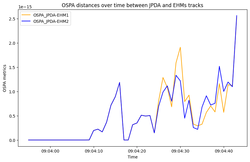
from stonesoup.metricgenerator.ospametric import OSPAMetric

ospa_JPDA_EHM1 = OSPAMetric(c=40, p=1, generator_name='OSPA_JPDA-EHM1',
                            tracks_key='JPDA_tracks', truths_key='EHM1_tracks')
ospa_JPDA_EHM2 = OSPAMetric(c=40, p=1, generator_name='OSPA_JPDA-EHM2',
                           tracks_key='JPDA_tracks', truths_key='EHM2_tracks')

# Define the track data associator
from stonesoup.dataassociator.tracktotrack import TrackToTruth

associator = TrackToTruth(association_threshold=30)

# Load the plotter
from stonesoup.metricgenerator.plotter import TwoDPlotter

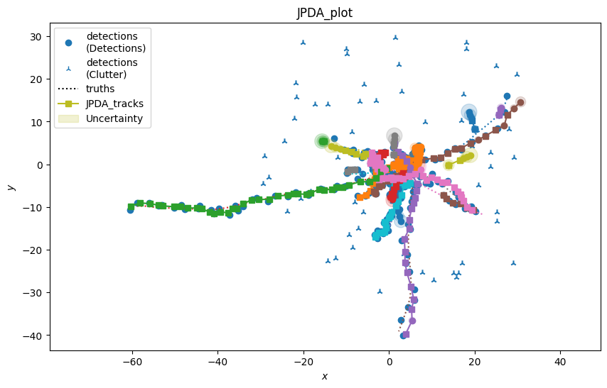
plot_generator_JPDA = TwoDPlotter([0, 2], [0, 2], [0, 2], uncertainty=True, tracks_key='JPDA_tracks',
                                 truths_key='truths', detections_key='detections',
                                 generator_name='JPDA_plot')
plot_generator_EHM1 = TwoDPlotter([0, 2], [0, 2], [0, 2], uncertainty=True, tracks_key='EHM1_tracks',
                                truths_key='truths', detections_key='detections',
                                generator_name='EHM1_plot')

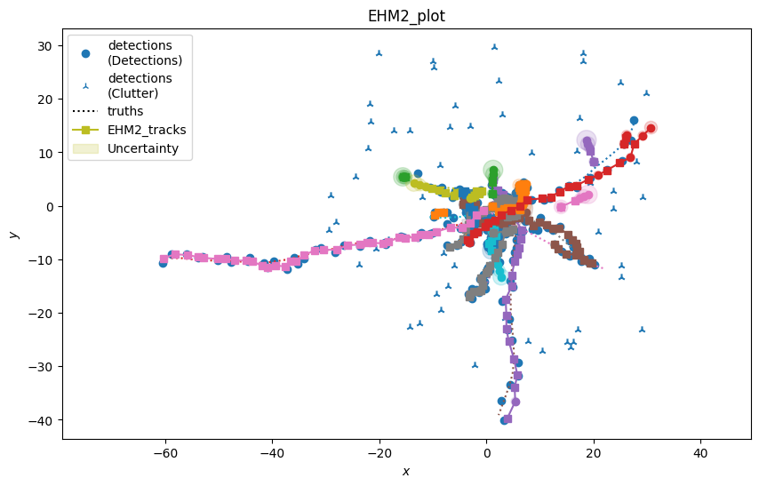
plot_generator_EHM2 = TwoDPlotter([0, 2], [0, 2], [0, 2], uncertainty=True, tracks_key='EHM2_tracks',
                                truths_key='truths', detections_key='detections',
                                generator_name='EHM2_plot')

# Load the multi-manager
from stonesoup.metricgenerator.manager import MultiManager

# Load all the relevant components of the plots in the metric manager
metric_manager = MultiManager([basic_JPDA,
                               EHM1,
                               EHM2,
                               ospa_JPDA_EHM1,
                               ospa_JPDA_EHM2,
                               plot_generator_JPDA,
                               plot_generator_EHM1,
                               plot_generator_EHM2
                               ], associator)

Run simulation

# We  plot the various tracker results
JPDA_tracks = set()
EHM1_tracks = set()
EHM2_tracks = set()
groundtruths = set()
detections_set = set()

# We measure the computation time
start_time = perf_counter()
for time, ctracks in JPDA_tracker:
    JPDA_tracks.update(ctracks)
    detections_set.update(detection_sim.detections)
jpda_time = perf_counter() - start_time

groundtruths = groundtruth_sim.groundtruth_paths

start_time = perf_counter()
for time, etracks in EHM1_tracker:
    EHM1_tracks.update(etracks)
ehm1_time = perf_counter() - start_time

start_time = perf_counter()
for time, etracks in EHM2_tracker:
    EHM2_tracks.update(etracks)
ehm2_time = perf_counter() - start_time

# Add the various tracks to the metric manager
metric_manager.add_data({'JPDA_tracks': JPDA_tracks}, overwrite=False)
metric_manager.add_data({'truths': groundtruths,
                        'detections': detections_set}, overwrite=False)
metric_manager.add_data({'EHM1_tracks': EHM1_tracks}, overwrite=False)
metric_manager.add_data({'EHM2_tracks': EHM2_tracks}, overwrite=False)

4) Compare the trackers performances

We have set up the trackers as well as the metric manager, to conclude this tutorial we show the results of the computing time needed for each tracker, the overall tracks generated and the differences between the tracks, if any. We start presenting the time performances of the different trackers along with the performance improvement obtained by the EHM data associators.

print('Comparisons between the trackers performances')
print(f'JPDA computing time: {jpda_time:.2f} seconds')
print(f'EHM1 computing time: {ehm1_time:.2f} seconds, {(jpda_time/ehm1_time-1)*100:.2f} % quicker than JPDA')
print(f'EHM2 computing time: {ehm2_time:.2f} seconds, {(jpda_time/ehm2_time-1)*100:.2f} % quicker than JPDA')

# Load the plotter package to plot the detections, tracks and detections.
from stonesoup.plotter import Plotterly

plotter = Plotterly()

plotter.plot_ground_truths(groundtruths, [0, 2])
plotter.plot_measurements(detections_set, [0, 2])
plotter.plot_tracks(JPDA_tracks, [0, 2], line= dict(color='orange'),
                    label='JPDA tracks')
plotter.plot_tracks(EHM1_tracks, [0, 2], line= dict(color='green', dash='dot'),
                    label='EHM1 tracks')
plotter.plot_tracks(EHM2_tracks, [0, 2], line= dict(color='red', dash='dot'),
                    label='EHM2 tracks')
plotter.fig

Comparisons between the trackers performances
JPDA computing time: 1.23 seconds
EHM1 computing time: 0.55 seconds, 121.37 % quicker than JPDA
EHM2 computing time: 0.55 seconds, 121.50 % quicker than JPDA

Show the metrics

# Now we process the metrics
metrics = metric_manager.generate_metrics()

# Load the metric plotter
from stonesoup.plotter import MetricPlotter
graph = MetricPlotter()

graph.plot_metrics(metrics, generator_names=['OSPA_JPDA-EHM1',
                                             'OSPA_JPDA-EHM2'],
                   color=['orange',  'blue'])

# update y-axis label and title, other subplots are displaying auto-generated title and labels
graph.axes[0].set(ylabel='OSPA metrics', title='OSPA distances over time between JPDA and EHMs tracks')
graph.fig
# Please note the scale of the plot

• 
• 
• 
• 

Conclusion

In this example we have shown how the performances of the tracker changes by employing or not an efficient management system. We measure a significant improvement (depending on the number of simulation steps, number of tracks and clutter rate) in the computation time in using EHM approaches compared to the brute force JPDA. The tracks obtained by the three trackers are perfectly aligned.

References

[1]

Maskell, S., Briers, M. and Wright, R., 2004, August. Fast mutual exclusion. In Signal and Data Processing of Small Targets 2004 (Vol. 5428, pp. 526-536). International Society for Optics and Photonics

[2]

Horridge, P. and Maskell, S., 2006, July. Real-time tracking of hundreds of targets with efficient exact JPDAF implementation. In 2006 9th International Conference on Information Fusion (pp. 1-8). IEEE