2 - Multiple Sensor Management

This tutorial follows on from the Single Sensor Management tutorial and further explores how existing Stone Soup features can be used to build simple sensor management algorithms for tracking and state estimation. This second tutorial demonstrates the limitations of the brute force optimisation method introduced in the previous tutorial by increasing the number of sensors used in the scenario.

Introducing multiple sensors

The example in this tutorial considers the same sensor management methods as in Tutorial 1 and applies them to the same set of ground truths in order to observe the difference in tracks. The scenario simulates 3 targets moving on nearly constant velocity trajectories and in this case an adjustable number of sensors. The sensors are simple radar with a defined field of view which can be pointed in a particular direction in order to make an observation.

The first method, using the class RandomSensorManager chooses a target for each sensor to observe randomly with equal probability.

The second method, uses the class BruteForceSensorManager and aims to reduce the total uncertainty of the track estimates at each time step. To achieve this the sensor manager considers all possible configurations of directions for the sensors to point in. The sensor manager chooses the configuration for which the sum of estimated uncertainties (as represented by the Frobenius norm of the covariance matrix) can be reduced the most by observing the targets within the chosen sensing configuration.

The introduction of multiple sensors means an increase in the possible combinations of action choices that the brute force sensor manager must consider. This brute force optimisation method of looking at every possible combination of actions becomes very slow as more sensors are introduced, demonstrating the limitations of using this method in more complex scenarios.

As in the first tutorial the OSPA 1, SIAP 2 and uncertainty metrics are used to assess the performance of the sensor managers.

Sensor Management example

Setup

First a simulation must be set up using components from Stone Soup. For this the following imports are required.

import numpy as np
import random
from datetime import datetime, timedelta

start_time = datetime.now()

from stonesoup.models.transition.linear import CombinedLinearGaussianTransitionModel, ConstantVelocity
from stonesoup.types.groundtruth import GroundTruthPath, GroundTruthState

Generate ground truths

Generate transition model and ground truths as in Tutorial 1.

The number of targets in this simulation is defined by ntruths - here there are 3 targets travelling in different directions. The time the simulation is observed for is defined by time_max.

We can fix our random number generator in order to probe a particular example repeatedly. This can be undone by commenting out the first two lines in the next cell.

np.random.seed(1990)
random.seed(1990)

# Generate transition model
transition_model = CombinedLinearGaussianTransitionModel([ConstantVelocity(0.005),
                                                          ConstantVelocity(0.005)])

yps = range(0, 100, 10)  # y value for prior state
truths = []
ntruths = 3  # number of ground truths in simulation
time_max = 50  # timestamps the simulation is observed over

xdirection = 1
ydirection = 1

# Generate ground truths
for j in range(0, ntruths):
    truth = GroundTruthPath([GroundTruthState([0, xdirection, yps[j], ydirection], timestamp=start_time)],
                            id=f"id{j}")

    for k in range(1, time_max):
        truth.append(
            GroundTruthState(transition_model.function(truth[k - 1], noise=True, time_interval=timedelta(seconds=1)),
                             timestamp=start_time + timedelta(seconds=k)))
    truths.append(truth)

    xdirection *= -1
    if j % 2 == 0:
        ydirection *= -1

Plot the ground truths. This is done using the Plotterly class from Stone Soup.

from stonesoup.plotter import Plotterly

# Stonesoup plotter requires sets not lists
truths_set = set(truths)

plotter = Plotterly()
plotter.plot_ground_truths(truths_set, [0, 2])
plotter.fig

Create sensors

Create a set of sensors for each sensor management algorithm. As in Tutorial 1 this tutorial uses the RadarRotatingBearingRange sensor with the number of sensors initially set as 2. Each sensor is positioned along the line \(x=10\), at distance intervals of 50.

Increasing the number of sensors above 2 significantly increases the run time of the sensor manager due to the increase in combinations to be considered by the BruteForceSensorManager. Note that in Tutorial 1 we did not set the resolution for the dwell centre whereas here we are setting it to 30 degrees. This is because for the brute force algorithm with multiple sensors, using the default resolution of 1 degree is not practical. These limitations due to combinatorics are discussed further later.

total_no_sensors = 2

from stonesoup.types.state import StateVector
from stonesoup.sensor.radar.radar import RadarRotatingBearingRange
from stonesoup.types.angle import Angle

sensor_setA = set()
for n in range(0, total_no_sensors):
    sensor = RadarRotatingBearingRange(
        position_mapping=(0, 2),
        noise_covar=np.array([[np.radians(0.5) ** 2, 0],
                              [0, 1 ** 2]]),
        ndim_state=4,
        position=np.array([[10], [n * 50]]),
        rpm=60,
        fov_angle=np.radians(30),
        dwell_centre=StateVector([0.0]),
        max_range=np.inf,
        resolutions={'dwell_centre': Angle(np.radians(30))}
    )
    sensor_setA.add(sensor)
for sensor in sensor_setA:
    sensor.timestamp = start_time

sensor_setB = set()
for n in range(0, total_no_sensors):
    sensor = RadarRotatingBearingRange(
        position_mapping=(0, 2),
        noise_covar=np.array([[np.radians(0.5) ** 2, 0],
                              [0, 1 ** 2]]),
        ndim_state=4,
        position=np.array([[10], [n * 50]]),
        rpm=60,
        fov_angle=np.radians(30),
        dwell_centre=StateVector([0.0]),
        max_range=np.inf,
        resolutions={'dwell_centre': Angle(np.radians(30))}
    )
    sensor_setB.add(sensor)

for sensor in sensor_setB:
    sensor.timestamp = start_time

Create the Kalman predictor and updater

Construct a predictor and updater using the KalmanPredictor and ExtendedKalmanUpdater components from Stone Soup. The measurement model for the updater is None as it is an attribute of the sensor.

from stonesoup.predictor.kalman import KalmanPredictor
predictor = KalmanPredictor(transition_model)

from stonesoup.updater.kalman import ExtendedKalmanUpdater
updater = ExtendedKalmanUpdater(measurement_model=None)
# measurement model is added to detections by the sensor

Run the Kalman filters

Create priors which estimate the targets’ initial states - these are the same as in the first sensor management tutorial.

from stonesoup.types.state import GaussianState

priors = []
xdirection = 1.2
ydirection = 1.2
for j in range(0, ntruths):
    priors.append(GaussianState([[0], [xdirection], [yps[j]+0.1], [ydirection]],
                                np.diag([0.5, 0.5, 0.5, 0.5]+np.random.normal(0,5e-4,4)),
                                timestamp=start_time))
    xdirection *= -1
    if j % 2 == 0:
        ydirection *= -1

Initialise the tracks by creating an empty list and appending the priors generated. This needs to be done separately for both sensor manager methods as they will generate different sets of tracks.

from stonesoup.types.track import Track

# Initialise tracks from the RandomSensorManager
tracksA = []
for j, prior in enumerate(priors):
    tracksA.append(Track([prior]))

# Initialise tracks from the BruteForceSensorManager
tracksB = []
for j, prior in enumerate(priors):
    tracksB.append(Track([prior]))

Create sensor managers

Next we create our sensor management classes. As in Tutorial 1, two sensor manager classes are used - RandomSensorManager and BruteForceSensorManager.

Random sensor manager

The first method RandomSensorManager, randomly chooses the action(s) for the sensors to take to make an observation. To do this the choose_actions() function uses random.choice() to choose a direction for each sensor to observe from the possible actions it can take. It returns the chosen configuration of sensors and actions to be taken as a mapping.

from stonesoup.sensormanager import RandomSensorManager

Brute force sensor manager

The second method BruteForceSensorManager chooses the configuration of sensors and actions which results in the greatest reward as calculated by the reward function.

In this example this is the largest difference between the uncertainty covariances of the target predictions and posteriors assuming a predicted measurement corresponding to that prediction. This means the sensor manager chooses to point the sensors in directions such that the uncertainty will be reduced the most by making observations in those directions.

from stonesoup.sensormanager import BruteForceSensorManager

Reward function

The UncertaintyRewardFunction calculates the uncertainty reduction by computing the difference between the covariance matrix norms of the prediction and the posterior assuming a predicted measurement corresponding to that prediction. The sum of these differences is returned as a metric for that configuration.

from stonesoup.sensormanager.reward import UncertaintyRewardFunction

Initiate sensor managers

Create an instance of each sensor manager class. Both sensor managers take in a sensor_set. The BruteForceSensorManager also requires a callable reward function which is initiated here from the UncertaintyRewardFunction.

randomsensormanager = RandomSensorManager(sensor_setA)

# initiate reward function
reward_function = UncertaintyRewardFunction(predictor, updater)

bruteforcesensormanager = BruteForceSensorManager(sensor_setB,
                                                  reward_function=reward_function)

Run the sensor managers

Both sensor management methods require a timestamp and a list of tracks at each time step when calling the function choose_actions(). This returns a mapping of sensors and actions to be taken by each sensor, decided by the sensor managers.

For both sensor management methods, at each time step the chosen action is given to the sensors and then measurements taken. The tracks are updated based on these measurements with predictions made for tracks which have not been observed.

First a hypothesiser and data associator are required for use in both trackers.

from stonesoup.hypothesiser.distance import DistanceHypothesiser
from stonesoup.measures import Mahalanobis
hypothesiser = DistanceHypothesiser(predictor, updater, measure=Mahalanobis(), missed_distance=5)

from stonesoup.dataassociator.neighbour import GNNWith2DAssignment
data_associator = GNNWith2DAssignment(hypothesiser)

Run random sensor manager

Here the chosen target for observation is selected randomly using the method choose_actions() from the class RandomSensorManager. This returns a mapping of sensors to actions where actions are a ChangeDwellAction, selected at random.

from ordered_set import OrderedSet

# Generate list of timesteps from ground truth timestamps
timesteps = []
for state in truths[0]:
    timesteps.append(state.timestamp)

for timestep in timesteps[1:]:

    # Generate chosen configuration
    chosen_actions = randomsensormanager.choose_actions(tracksA, timestep)

    # Create empty dictionary for measurements
    measurementsA = []

    for chosen_action in chosen_actions:
        for sensor, actions in chosen_action.items():
            sensor.add_actions(actions)

    for sensor in sensor_setA:
        sensor.act(timestep)

        # Observe this ground truth
        measurements = sensor.measure(OrderedSet(truth[timestep] for truth in truths), noise=True)
        measurementsA.extend(measurements)

    hypotheses = data_associator.associate(tracksA,
                                           measurementsA,
                                           timestep)
    for track in tracksA:
        hypothesis = hypotheses[track]
        if hypothesis.measurement:
            post = updater.update(hypothesis)
            track.append(post)
        else:  # When data associator says no detections are good enough, we'll keep the prediction
            track.append(hypothesis.prediction)

Plot ground truths, tracks and uncertainty ellipses for each target. The positions of the sensors are indicated by black x markers.

plotterA = Plotterly()
plotterA.plot_sensors(sensor_setA)
plotterA.plot_ground_truths(truths_set, [0, 2])
plotterA.plot_tracks(set(tracksA), [0, 2], uncertainty=True)
plotterA.fig

In comparison to Tutorial 1 the performance of the RandomSensorManager has improved. This is because a greater number of sensors means each target is more likely to be observed. This means the uncertainty of the track does not increase as much because the targets are observed more often.

Run brute force sensor manager

Here the direction for observation is selected based on the difference between the covariance matrices of the prediction and posterior, for targets which could be observed by the sensor pointing in the given direction.

Within the sensor manager a dictionary is created of sensors and all the possible actions they can take. When the choose_actions() function is called (at each time step), for each track in the tracks list:

• A prediction is made for each track and the covariance matrix norms stored

• For each possible action a sensor could take, a synthetic detection is made using this sensor configuration

• A hypothesis is generated based on the stored prediction and synthetic detection

• This hypothesis is used to do an update and the covariance matrix norms of the update are stored

• The difference between the covariance matrix norms of the update and the prediction is calculated

The overall reward is calculated as the sum of the differences between these covariance matrix norms for the tracks observed by the possible action configuration. The sensor manager identifies the configuration which results in the largest value of this reward and therefore largest reduction in uncertainty. It returns the optimum sensors/actions configuration as a dictionary.

The actions are given to the sensors, measurements made and the tracks updated based on these measurements. Predictions are made for tracks which have not been observed by the sensors.

for timestep in timesteps[1:]:

    # Generate chosen configuration
    chosen_actions = bruteforcesensormanager.choose_actions(tracksB, timestep)

    # Create empty dictionary for measurements
    measurementsB = []

    for chosen_action in chosen_actions:
        for sensor, actions in chosen_action.items():
            sensor.add_actions(actions)

    for sensor in sensor_setB:
        sensor.act(timestep)

        # Observe this ground truth
        measurements = sensor.measure(OrderedSet(truth[timestep] for truth in truths), noise=True)
        measurementsB.extend(measurements)

    hypotheses = data_associator.associate(tracksB,
                                           measurementsB,
                                           timestep)
    for track in tracksB:
        hypothesis = hypotheses[track]
        if hypothesis.measurement:
            post = updater.update(hypothesis)
            track.append(post)
        else:  # When data associator says no detections are good enough, we'll keep the prediction
            track.append(hypothesis.prediction)

Plot ground truths, tracks and uncertainty ellipses for each target.

plotterB = Plotterly()
plotterB.plot_sensors(sensor_setB)
plotterB.plot_ground_truths(truths_set, [0, 2])
plotterB.plot_tracks(set(tracksB), [0, 2], uncertainty=True)
plotterB.fig

The smaller uncertainty ellipses in this plot suggest that the BruteForceSensorManager provides a much better track than the RandomSensorManager. The tracking is also improved from Tutorial 1 due to the increased number of sensors.

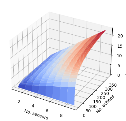
Combinatorics

The following graph demonstrates how the number of possible sensor-action configurations increases with the number of sensors and number of actions. The number of configurations which are considered by the sensor manager for \(M\) actions and \(N\) sensors is \(M^N\).

With a resolution of 1 degree there are 360 possible dwell centres for a sensor so the number of possible configurations should be \(360^N\) where \(N\) is the number of sensors. This exponential increase means that as the number of sensors increase, the run time of the sensor manager slows down significantly because there are so many more iterations to consider.

In this scenario \(N=2\) so with a resolution of 1 degree that would 129,600 actions to consider. Even with a resolution of 30 degrees, changing the number of sensors to \(N\geq 2\) leads to a much longer run time. This highlights a practical limitation of using this brute force optimisation method for multiple sensors. In this example we have dealt with this by introducing a run time limit to the brute force sensor manager.

import matplotlib.pyplot as plt

nsensors = np.arange(1, 10)
nactions = np.arange(1, 360.0)
nsensors, nactions = np.meshgrid(nsensors, nactions)
ncombinations = nactions**nsensors

fig = plt.figure()
ax = fig.add_subplot(projection="3d")
ax.plot_surface(nsensors, nactions, np.log10(ncombinations), cmap='coolwarm')
ax.set_xlabel("No. sensors")
ax.set_ylabel("No. actions")
ax.set_zlabel("log of no. combinations")

Text(0.10787434422876356, 0.014452421710067023, 'log of no. combinations')

Metrics

Metrics can be used to compare how well different sensor management techniques are working. As in Tutorial 1 the metrics used here are the OSPA, SIAP and uncertainty metrics.

from stonesoup.metricgenerator.ospametric import OSPAMetric
ospa_generator = OSPAMetric(c=40, p=1)

from stonesoup.metricgenerator.tracktotruthmetrics import SIAPMetrics
from stonesoup.measures import Euclidean
siap_generator = SIAPMetrics(position_measure=Euclidean((0, 2)),
                             velocity_measure=Euclidean((1, 3)))

from stonesoup.dataassociator.tracktotrack import TrackToTruth
associator = TrackToTruth(association_threshold=30)

from stonesoup.metricgenerator.uncertaintymetric import SumofCovarianceNormsMetric
uncertainty_generator = SumofCovarianceNormsMetric()

Generate a metrics manager for each sensor management method.

from stonesoup.metricgenerator.manager import SimpleManager

metric_managerA = SimpleManager([ospa_generator, siap_generator, uncertainty_generator],
                                associator=associator)

metric_managerB = SimpleManager([ospa_generator, siap_generator, uncertainty_generator],
                                associator=associator)

For each time step, data is added to the metric manager on truths and tracks. The metrics themselves can then be generated from the metric manager.

metric_managerA.add_data(truths, tracksA)
metric_managerB.add_data(truths, tracksB)

metricsA = metric_managerA.generate_metrics()
metricsB = metric_managerB.generate_metrics()

OSPA metric

First we look at the OSPA metric. This is plotted over time for each sensor manager method.

ospa_metricA = metricsA['OSPA distances']
ospa_metricB = metricsB['OSPA distances']

fig = plt.figure()
ax = fig.add_subplot(1, 1, 1)
ax.plot([i.timestamp for i in ospa_metricA.value],
        [i.value for i in ospa_metricA.value],
        label='RandomSensorManager')
ax.plot([i.timestamp for i in ospa_metricB.value],
        [i.value for i in ospa_metricB.value],
        label='BruteForceSensorManager')
ax.set_ylabel("OSPA distance")
ax.set_xlabel("Time")
ax.legend()

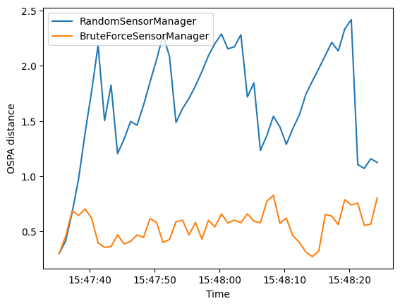
The OSPA distance for the BruteForceSensorManager is generally smaller than for the random observations of the RandomSensorManager.

SIAP metrics

Next we look at SIAP metrics. We are only interested in the positional accuracy (PA) and velocity accuracy (VA). These metrics can be plotted to show how they change over time.

fig, axes = plt.subplots(2)

times = metric_managerA.list_timestamps()

pa_metricA = metricsA['SIAP Position Accuracy at times']
va_metricA = metricsA['SIAP Velocity Accuracy at times']

pa_metricB = metricsB['SIAP Position Accuracy at times']
va_metricB = metricsB['SIAP Velocity Accuracy at times']

axes[0].set(title='Positional Accuracy', xlabel='Time', ylabel='PA')
axes[0].plot(times, [metric.value for metric in pa_metricA.value],
             label='RandomSensorManager')
axes[0].plot(times, [metric.value for metric in pa_metricB.value],
             label='BruteForceSensorManager')
axes[0].legend()

axes[1].set(title='Velocity Accuracy', xlabel='Time', ylabel='VA')
axes[1].plot(times, [metric.value for metric in va_metricA.value],
             label='RandomSensorManager')
axes[1].plot(times, [metric.value for metric in va_metricB.value],
             label='BruteForceSensorManager')
axes[1].legend()

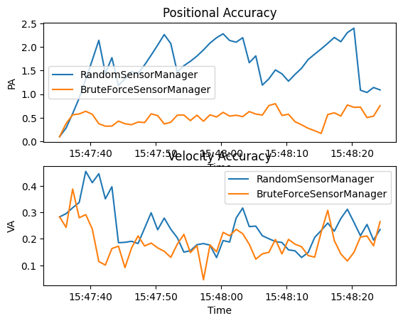
Similar to the OSPA distance the BruteForceSensorManager generally results in both a better positional accuracy and velocity accuracy than the random observations of the RandomSensorManager.

Uncertainty metric

Finally we look at the uncertainty metric which computes the sum of covariance matrix norms of each state at each time step. This is plotted over time for each sensor manager method.

uncertainty_metricA = metricsA['Sum of Covariance Norms Metric']
uncertainty_metricB = metricsB['Sum of Covariance Norms Metric']

fig = plt.figure()
ax = fig.add_subplot(1, 1, 1)
ax.plot([i.timestamp for i in uncertainty_metricA.value],
        [i.value for i in uncertainty_metricA.value],
        label='RandomSensorManager')
ax.plot([i.timestamp for i in uncertainty_metricB.value],
        [i.value for i in uncertainty_metricB.value],
        label='BruteForceSensorManager')
ax.set_ylabel("Sum of covariance matrix norms")
ax.set_xlabel("Time")
ax.legend()

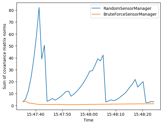
This metric shows that the uncertainty in the tracks generated by the RandomSensorManager is generally greater than for those generated by the BruteForceSensorManager. This is also reflected by the uncertainty ellipses in the initial plots of tracks and truths.

References

1

D. Schuhmacher, B. Vo and B. Vo, A Consistent Metric for Performance Evaluation of Multi-Object Filters, IEEE Trans. Signal Processing 2008

2

Votruba, Paul & Nisley, Rich & Rothrock, Ron and Zombro, Brett., Single Integrated Air Picture (SIAP) Metrics Implementation, 2001