Video processing, Object detection & Tracking

Demonstrating the video processing capabilities of Stone Soup

This notebook will guide you progressively through the steps necessary to:

1. Use the Stone Soup FrameReader components to open and process video data;

2. Use the UltralyticsBoxObjectDetector to detect objects in video data, making use of Ultralytics YOLO object detection models;

3. Build a MultiTargetTracker to perform tracking of multiple object in video data.

Software dependencies

Before we begin with this tutorial, there are a few things that we need to install in order to proceed.

FFmpeg

FFmpeg is a free and open-source project consisting of a vast software suite of libraries and programs for handling video, audio, and other multimedia files and streams. Stone Soup (or more accurately some of its extra dependencies) make use of FFmpeg to read and output video. Download links and installation instructions for FFmpeg can be found here.

Ultralytics

Ultralytics is a free and open-source library that provides an easy-to-use interface to the YOLO family of object detection models. It ships with a collection of pre-trained models that can be used for out-of-the-box inference, and downloads the requested model weights automatically on first use. Installation instructions can be found in the Ultralytics quickstart guide.

Stone Soup

To perform video-processing using Stone Soup, we need to install some extra dependencies. The easiest way to achieve this is by running the following commands in a Terminal window:

git clone "https://github.com/dstl/Stone-Soup.git"
cd Stone-Soup
python -m pip install -e .[dev,video,ultralytics]

yt-dlp

We will also use yt-dlp to download a YouTube video for the purposes of this tutorial. This is installed as part of the video extra above, but can also be installed on its own by running the following command in the same Terminal window:

pip install yt-dlp

Using the Stone Soup FrameReader classes

The FrameReader abstract class is intended as the base class for Stone Soup readers that read frames from any form of imagery data. As of now, Stone Soup has two implementations of FrameReader subclasses:

1. The VideoClipReader component, which uses MoviePy to read video frames from a file.

2. The FFmpegVideoStreamReader component, which uses ffmpeg-python to read frames from real-time video streams (e.g. RTSP).

In this tutorial we will focus on the VideoClipReader, since setting up a stream for the FFmpegVideoStreamReader is more involved. Nevertheless, the use and interface of the two readers is mostly identical after initialisation and an example of how to initialise the later will also be provided

Download and store the video

First we will download the video that we will use throughout this tutorial. The code snippet shown below will download the video and save it your working directory as sample1.mp4.

import os
import yt_dlp
VIDEO_FILENAME = 'sample1'
VIDEO_EXTENTION = '.mp4'
VIDEO_PATH = os.path.join(os.getcwd(), VIDEO_FILENAME+VIDEO_EXTENTION)

if not os.path.exists(VIDEO_PATH):
    ydl_opts = {'outtmpl': VIDEO_PATH, 'format': '18'}  # format 18 is 360p mp4
    with yt_dlp.YoutubeDL(ydl_opts) as ydl:
        ydl.download(['https://www.youtube.com/watch?v=MNn9qKG2UFI'])

[youtube] Extracting URL: https://www.youtube.com/watch?v=MNn9qKG2UFI
[youtube] MNn9qKG2UFI: Downloading webpage
[youtube] MNn9qKG2UFI: Downloading android vr player API JSON
[info] MNn9qKG2UFI: Downloading 1 format(s): 18

[download]   0.0% of   20.91MiB at  Unknown B/s ETA Unknown
[download]   0.0% of   20.91MiB at    1.86MiB/s ETA 00:11
[download]   0.0% of   20.91MiB at    1.88MiB/s ETA 00:11
[download]   0.1% of   20.91MiB at    3.44MiB/s ETA 00:06
[download]   0.1% of   20.91MiB at    3.51MiB/s ETA 00:05
[download]   0.3% of   20.91MiB at    4.56MiB/s ETA 00:04
[download]   0.6% of   20.91MiB at    2.63MiB/s ETA 00:07
[download]   1.2% of   20.91MiB at    2.63MiB/s ETA 00:07
[download]   2.4% of   20.91MiB at    3.21MiB/s ETA 00:06
[download]   4.8% of   20.91MiB at    3.86MiB/s ETA 00:05
[download]   9.6% of   20.91MiB at    5.15MiB/s ETA 00:03
[download]  19.1% of   20.91MiB at    6.64MiB/s ETA 00:02
[download]  38.3% of   20.91MiB at    8.48MiB/s ETA 00:01
[download]  46.8% of   20.91MiB at    9.09MiB/s ETA 00:01
[download]  46.8% of   20.91MiB at  Unknown B/s ETA Unknown
[download]  46.8% of   20.91MiB at    2.41MiB/s ETA 00:04
[download]  46.9% of   20.91MiB at    4.33MiB/s ETA 00:02
[download]  46.9% of   20.91MiB at    7.63MiB/s ETA 00:01
[download]  47.0% of   20.91MiB at    3.30MiB/s ETA 00:03
[download]  47.1% of   20.91MiB at    4.30MiB/s ETA 00:02
[download]  47.4% of   20.91MiB at    4.27MiB/s ETA 00:02
[download]  48.0% of   20.91MiB at    4.40MiB/s ETA 00:02
[download]  49.2% of   20.91MiB at    5.17MiB/s ETA 00:02
[download]  51.6% of   20.91MiB at    6.14MiB/s ETA 00:01
[download]  56.4% of   20.91MiB at    6.81MiB/s ETA 00:01
[download]  66.0% of   20.91MiB at    8.12MiB/s ETA 00:00
[download]  85.1% of   20.91MiB at    9.79MiB/s ETA 00:00
[download]  93.5% of   20.91MiB at   10.11MiB/s ETA 00:00
[download]  93.5% of   20.91MiB at  Unknown B/s ETA Unknown
[download]  93.5% of   20.91MiB at    2.22MiB/s ETA 00:00
[download]  93.5% of   20.91MiB at    3.71MiB/s ETA 00:00
[download]  93.5% of   20.91MiB at    6.63MiB/s ETA 00:00
[download]  93.6% of   20.91MiB at    4.87MiB/s ETA 00:00
[download]  93.7% of   20.91MiB at    4.47MiB/s ETA 00:00
[download]  94.0% of   20.91MiB at    4.94MiB/s ETA 00:00
[download]  94.6% of   20.91MiB at    4.07MiB/s ETA 00:00
[download]  95.8% of   20.91MiB at    5.25MiB/s ETA 00:00
[download]  98.2% of   20.91MiB at    6.15MiB/s ETA 00:00
[download] 100.0% of   20.91MiB at    5.35MiB/s ETA 00:00
[download] 100% of   20.91MiB in 00:00:02 at 7.79MiB/s

Building the video reader

VideoClipReader

We will use the VideoClipReader class to read and replay the downloaded file. We also configure the reader to only replay the clip for the a duration of 2 seconds between 00:10 and 00:12.

import datetime
from stonesoup.reader.video import VideoClipReader
start_time = datetime.timedelta(minutes=0, seconds=10)
end_time = datetime.timedelta(minutes=0, seconds=12)
frame_reader = VideoClipReader(VIDEO_PATH, start_time, end_time)

It is also possible to apply clip transformations and effects, as per the MoviePy documentation. The underlying MoviePy VideoFileClip instance can be accessed through the clip class property. For example, we can crop out 100 pixels from the top and left of the frames, as they are read by the reader, as shown below.

frame_reader.clip = frame_reader.clip.cropped(x1=100, y1=100)
num_frames = len(list(frame_reader.clip.iter_frames()))

FFmpegVideoStreamReader

For reference purposes, we also include here an example of how to build a FFmpegVideoStreamReader. Let’s assume that we have a camera which broadcasts its feed through a public RTSP stream, under the URL rtsp://192.168.55.10:554/stream. We can build a FFmpegVideoStreamReader object to read frames from this stream as follows:

in_opts = {'threads': 1, 'fflags': 'nobuffer'}
out_opts = {'format': 'rawvideo', 'pix_fmt': 'bgr24'}
stream_url = 'rtsp://192.168.55.10:554/stream'
video_reader = FFmpegVideoStreamReader(stream_url, input_opts=in_opts, output_opts=out_opts)

Important

Note that the above code is an illustrative example and will not be run.

input_opts and output_opts are optional arguments, which allow users to specify options for the input and output FFmpeg streams, as documented by FFmpeg and ffmpeg-python.

Reading frames from the reader

All FrameReader objects, of which the VideoClipReader is a subclass, generate frames in the form of ImageFrame objects. Below we show an example of how to read and visualise these frames using matplotlib.

from copy import copy
from PIL import Image
from matplotlib import pyplot as plt
from matplotlib import animation

fig, ax = plt.subplots(num="VideoClipReader output")
artists = []

print('Running FrameReader example...')
for timestamp, frame in frame_reader:
    if not (len(artists)+1) % 10:
        print("Frame: {}/{}".format(len(artists)+1, num_frames))

    # Read the frame pixels
    pixels = copy(frame.pixels)

    # Plot output
    image = Image.fromarray(pixels)
    ax.axes.xaxis.set_visible(False)
    ax.axes.yaxis.set_visible(False)
    fig.tight_layout()
    artist = ax.imshow(image, animated=True)
    artists.append([artist])

ani = animation.ArtistAnimation(fig, artists, interval=20, blit=True, repeat_delay=200)

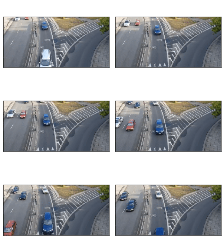
Running FrameReader example...
Frame: 10/60
Frame: 20/60
Frame: 30/60
Frame: 40/60
Frame: 50/60
Frame: 60/60

Using the UltralyticsBoxObjectDetector class

We now continue by demonstrating how to use the UltralyticsBoxObjectDetector to detect objects, and more specifically cars, within the frames read in by our frame_reader. The UltralyticsBoxObjectDetector can utilise both pre-trained and custom-trained Ultralytics YOLO models which generate detections in the form of bounding boxes. In this example, we will make use of a small pre-trained model, but the process of using a custom-trained YOLO model is the same.

The model

Unlike some other object detection frameworks, Ultralytics handles model management for us: when we reference a pre-trained model by name (e.g. yolo11n.pt), the corresponding weights are downloaded automatically the first time they are required and cached for subsequent runs. There is therefore no need to manually download a model or a separate label file.

The particular model we will use is YOLO11 in its smallest (nano) configuration, pre-trained on the MS COCO dataset. Larger variants (e.g. yolo11s.pt, yolo11m.pt) trade inference speed for accuracy.

Building the detector

Next, we proceed to initialise our detector object. To do this, we require the frame_reader object we built previously, as well as the name (or path) of the YOLO model we wish to use.

The UltralyticsBoxObjectDetector object can optionally be configured to digest frames from the provided reader asynchronously, and only perform detection on the last frame digested, by setting run_async=True. This is suitable when the detector is applied to readers generating a live feed (e.g. the FFmpegVideoStreamReader), where real-time processing is paramount. Since we are using a VideoClipReader in this example, we set run_async=False, which is also the default setting.

from stonesoup.detector.ultralytics import UltralyticsBoxObjectDetector

run_async = False                           # Configure the detector to run in synchronous mode
detector = UltralyticsBoxObjectDetector(frame_reader, 'yolo11n.pt', run_async=run_async)

Downloading https://github.com/ultralytics/assets/releases/download/v8.4.0/yolo11n.pt to 'yolo11n.pt': 11% ━─────────── 608.0KB/5.4MB 5.9MB/s 0.1s<0.8s
Downloading https://github.com/ultralytics/assets/releases/download/v8.4.0/yolo11n.pt to 'yolo11n.pt': 24% ━━╸───────── 1.3/5.4MB 7.3MB/s 0.2s<0.6s
Downloading https://github.com/ultralytics/assets/releases/download/v8.4.0/yolo11n.pt to 'yolo11n.pt': 39% ━━━━╸─────── 2.1/5.4MB 7.7MB/s 0.3s<0.4s
Downloading https://github.com/ultralytics/assets/releases/download/v8.4.0/yolo11n.pt to 'yolo11n.pt': 59% ━━━━━━━───── 3.2/5.4MB 10.0MB/s 0.4s<0.2s
Downloading https://github.com/ultralytics/assets/releases/download/v8.4.0/yolo11n.pt to 'yolo11n.pt': 77% ━━━━━━━━━─── 4.1/5.4MB 9.4MB/s 0.5s<0.1s
Downloading https://github.com/ultralytics/assets/releases/download/v8.4.0/yolo11n.pt to 'yolo11n.pt': 99% ━━━━━━━━━━━╸ 5.3/5.4MB 7.8MB/s 0.7s<0.0s
Downloading https://github.com/ultralytics/assets/releases/download/v8.4.0/yolo11n.pt to 'yolo11n.pt': 100% ━━━━━━━━━━━━ 5.4MB 8.0MB/s 0.7s

Filtering-out unwanted detections

In this section we showcase how we can utilise Stone Soup Feeder objects in order to filter out unwanted detections. One example of feeder we can use is the MetadataValueFilter, which allows us to filter detections by applying a custom operator on particular fields of the metadata property of detections.

Each detection generated by UltralyticsBoxObjectDetector carries the following metadata fields:

• raw_box: The raw bounding box containing the normalised coordinates [y_0, x_0, y_1, x_1].

• class: A dict with keys id and name relating to the id and name of the detection class.

• score: A float in the range (0, 1] indicating the detector’s confidence.

Detection models trained on the MS COCO dataset, such as the one we are using, are able to detect 80 different classes of objects (see the Ultralytics COCO documentation for a full list). Instead, as we discussed at the beginning of the tutorial, we wish to limit the detections to only those classified as cars. This can be done as follows:

from stonesoup.feeder.filter import MetadataValueFilter
detector = MetadataValueFilter(detector, 'class', lambda x: x['name'] == 'car')

Continuing, we may want to filter out detections which have a low confidence score:

detector = MetadataValueFilter(detector, 'score', lambda x: x > 0.1)

Finally, we observed that the detector tends to incorrectly generate detections which are much larger the the size we expect for a car. Therefore, we can filter out those detections by only allowing ones whose width is less the 20% of the frame width (i.e. x_1-x_0 < 0.2):

detector = MetadataValueFilter(detector, 'raw_box', lambda x: x[3]-x[1] < 0.2)

You are encouraged to comment out any/all of the above filter definitions and observe the produced output.

Reading and visualising detections

Detections generated by the UltralyticsBoxObjectDetector have a 4-dimensional state_vector in the form of a bounding boxes that captures the area of the frame where an object is detected. Each bounding box is represented by a vector of the form [x, y, w, h], where x, y denote the relative pixel coordinates of the top-left corner, while w, h denote the relative width and height of the bounding box. Below we show an example of how to read and visualise these detections using matplotlib.

import numpy as np
from PIL import ImageDraw


def draw_detections(image, detections, show_class=False, show_score=False):
    """ Draw detections on an image

    Parameters
    ----------
    image: :class:`PIL.Image`
        Image on which to draw the detections
    detections: : set of :class:`~.Detection`
        A set of detections generated by :class:`~.UltralyticsBoxObjectDetector`
    show_class: bool
        Whether to draw the class of the object. Default is ``False``
    show_score: bool
        Whether to draw the score of the object. Default is ``False``

    Returns
    -------
    : :class:`PIL.Image`
        Image with detections drawn
    """
    draw = ImageDraw.Draw(image)
    for detection in detections:
        x0, y0, w, h = np.array(detection.state_vector).reshape(4)
        x1, y1 = (x0 + w, y0 + h)
        draw.rectangle([x0, y0, x1, y1], outline=(0, 255, 0), width=1)
        class_ = detection.metadata['class']['name']
        score = round(float(detection.metadata['score']),2)
        if show_class and show_score:
            draw.text((x0,y1 + 2), '{}:{}'.format(class_, score), fill=(0, 255, 0))
        elif show_class:
            draw.text((x0, y1 + 2), '{}'.format(class_), fill=(0, 255, 0))
        elif show_score:
            draw.text((x0, y1 + 2), '{}'.format(score), fill=(0, 255, 0))

    del draw
    return image


fig2, ax2 = plt.subplots(num="UltralyticsBoxObjectDetector output")
artists2 = []
print("Running UltralyticsBoxObjectDetector example... Be patient...")
for timestamp, detections in detector:
    if not (len(artists2)+1) % 10:
        print("Frame: {}/{}".format(len(artists2)+1, num_frames))

    # Read the frame pixels
    frame = frame_reader.frame
    pixels = copy(frame.pixels)

    # Plot output
    image = Image.fromarray(pixels)
    image = draw_detections(image, detections, True, True)
    ax2.axes.xaxis.set_visible(False)
    ax2.axes.yaxis.set_visible(False)
    fig2.tight_layout()
    artist = ax2.imshow(image, animated=True)
    artists2.append([artist])

ani2 = animation.ArtistAnimation(fig2, artists2, interval=20, blit=True, repeat_delay=200)

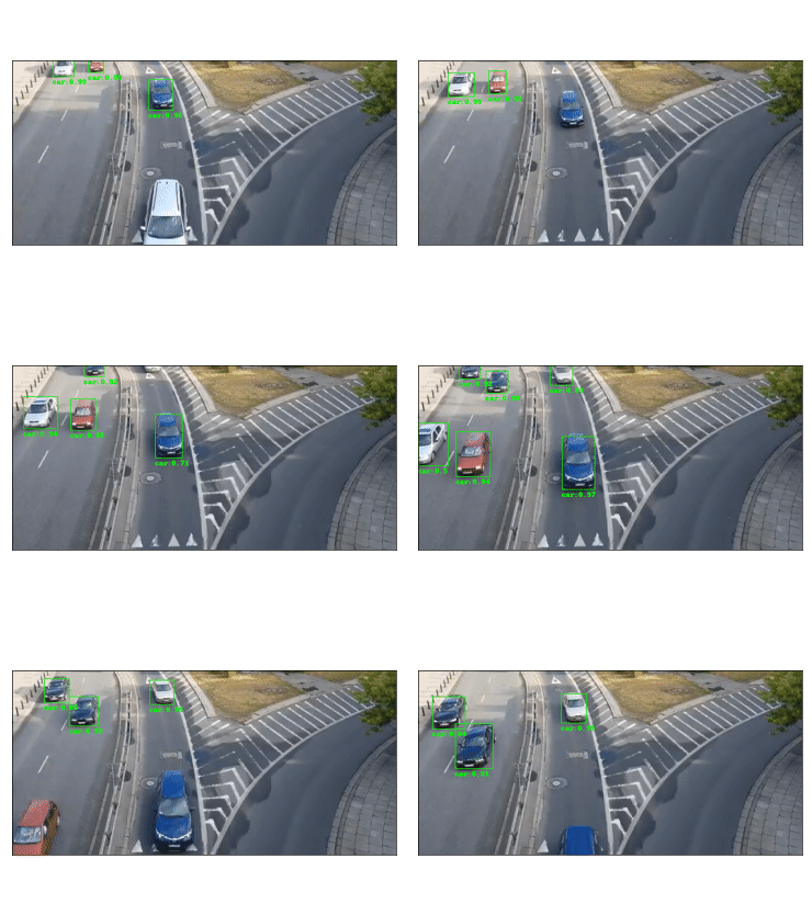
Running UltralyticsBoxObjectDetector example... Be patient...
Frame: 10/60
Frame: 20/60
Frame: 30/60
Frame: 40/60
Frame: 50/60
Frame: 60/60

Constructing a Multi-Object Video Tracker

In this final segment of the tutorial we will see how we can use the above demonstrated components to perform tracking of multiple objects within Stone Soup.

Defining the state-space models

Transition Model

We begin our definition of the state-space models by defining the hidden state \(\mathrm{x}_k\), i.e. the state that we wish to estimate:

\[\mathrm{x}_k = [x_k, \dot{x}_k, y_k, \dot{y}_k, w_k, h_k]\]

where \(x_k, y_k\) denote the pixel coordinates of the top-left corner of the bounding box containing an object, with \(\dot{x}_k, \dot{y}_k\) denoting their respective rate of change, while \(w_k\) and \(h_k\) denote the width and height of the box, respectively.

We assume that \(x_k\) and \(y_k\) move with nearly ConstantVelocity, while \(w_k\) and \(h_k\) evolve according to a RandomWalk.Using these assumptions, we proceed to construct our Stone Soup TransitionModel as follows:

from stonesoup.models.transition.linear import (CombinedLinearGaussianTransitionModel,
                                                ConstantVelocity, RandomWalk)
t_models = [ConstantVelocity(20**2), ConstantVelocity(20**2), RandomWalk(20**2), RandomWalk(20**2)]
transition_model = CombinedLinearGaussianTransitionModel(t_models)

Measurement Model

Continuing, we define the measurement state \(\mathrm{y}_k\), which follows naturally from the form of the detections generated by the UltralyticsBoxObjectDetector we previously discussed:

\[\mathrm{y}_k = [x_k, y_k, w_k, h_k]\]

We make use of a 4-dimensional LinearGaussian model as our MeasurementModel, whereby we can see that the individual indices of \(\mathrm{y}_k\) map to indices [0,2,4,5] of the 6-dimensional state \(\mathrm{x}_k\):

from stonesoup.models.measurement.linear import LinearGaussian
measurement_model = LinearGaussian(ndim_state=6, mapping=[0, 2, 4, 5],
                                   noise_covar=np.diag([1**2, 1**2, 3**2, 3**2]))

Defining the tracker components

With the state-space models defined, we proceed to build our tracking components

Filtering

Since we have assumed Linear-Gaussian models, we will be using a Kalman Filter to perform filtering of the underlying single-target densities. This is done by making use of the KalmanPredictor and KalmanUpdater classes, which we define below:

from stonesoup.predictor.kalman import KalmanPredictor
predictor = KalmanPredictor(transition_model)

from stonesoup.updater.kalman import KalmanUpdater
updater = KalmanUpdater(measurement_model)

Note

For more information on the above classes and how they operate you can refer to the Stone Soup tutorial on using the Kalman Filter.

Data Association

We utilise a DistanceHypothesiser to generate hypotheses between tracks and measurements, where Mahalanobis distance is used as a measure of quality:

from stonesoup.hypothesiser.distance import DistanceHypothesiser
from stonesoup.measures import Mahalanobis
hypothesiser = DistanceHypothesiser(predictor, updater, Mahalanobis(), 10)

Continuing the GNNWith2DAssigment class is used to perform fast joint data association, based on the Global Nearest Neighbour (GNN) algorithm:

from stonesoup.dataassociator.neighbour import GNNWith2DAssignment
data_associator = GNNWith2DAssignment(hypothesiser)

Note

For more information on the above classes and how they operate you can refer to the Data Association - clutter and Data Association - Multi-Target Tracking tutorials.

Track Initiation

For initialising tracks we will use a MultiMeasurementInitiator, which allows our tracker to tentatively initiate tracks from unassociated measurements, and hold them within the initiator until they have survived for at least 10 frames. We also define a UpdateTimeStepsDeleter deleter to be used by the initiator to delete tentative tracks that have not been associated to a measurement in the last 3 frames.

from stonesoup.types.state import GaussianState
from stonesoup.types.array import CovarianceMatrix, StateVector
from stonesoup.initiator.simple import MultiMeasurementInitiator
from stonesoup.deleter.time import UpdateTimeStepsDeleter
prior_state = GaussianState(StateVector(np.zeros((6,1))),
                            CovarianceMatrix(np.diag([100**2, 30**2, 100**2, 30**2, 100**2, 100**2])))
deleter_init = UpdateTimeStepsDeleter(time_steps_since_update=3)
initiator = MultiMeasurementInitiator(prior_state, deleter_init, data_associator, updater,
                                      measurement_model, min_points=10)

Track Deletion

For confirmed tracks we used again a UpdateTimeStepsDeleter, but this time configured to delete tracks after they have not bee associated to a measurement in the last 15 frames.

deleter = UpdateTimeStepsDeleter(time_steps_since_update=15)

Note

For more information on the above classes and how they operate you can refer to the Stone Initiators & Deleters tutorial.

Building the tracker

Now that we have defined all our tracker components we proceed to build our multi-target tracker:

from stonesoup.tracker.simple import MultiTargetTracker
tracker = MultiTargetTracker(
    initiator=initiator,
    deleter=deleter,
    detector=detector,
    data_associator=data_associator,
    updater=updater,
)

Running the tracker

def draw_tracks(image, tracks, show_history=True, show_class=True, show_score=True):
    """ Draw tracks on an image

    Parameters
    ----------
    image: :class:`PIL.Image`
        Image on which to draw the tracks
    detections: : set of :class:`~.Tracks`
        A set of tracks generated by our :class:`~.MultiTargetTracker`
    show_history: bool
        Whether to draw the trajectory of the track. Default is ``True``
    show_class: bool
        Whether to draw the class of the object. Default is ``True``
    show_score: bool
        Whether to draw the score of the object. Default is ``True``

    Returns
    -------
    : :class:`PIL.Image`
        Image with tracks drawn

    """
    draw = ImageDraw.Draw(image)
    for track in tracks:
        bboxes = np.array([np.array(state.state_vector[[0, 2, 4, 5]]).reshape(4)
                           for state in track.states])
        x0, y0, w, h = bboxes[-1]
        x1 = x0 + w
        y1 = y0 + h
        draw.rectangle([x0, y0, x1, y1], outline=(255, 0, 0), width=2)

        if show_history:
            pts = [(box[0] + box[2] / 2, box[1] + box[3] / 2) for box in bboxes]
            draw.line(pts, fill=(255, 0, 0), width=2)

        class_ = track.metadata['class']['name']
        score = round(float(track.metadata['score']), 2)
        if show_class and show_score:
            draw.text((x0, y1 + 2), '{}:{}'.format(class_, score), fill=(255, 0, 0))
        elif show_class:
            draw.text((x0, y1 + 2), '{}'.format(class_), fill=(255, 0, 0))
        elif show_score:
            draw.text((x0, y1 + 2), '{}'.format(score), fill=(255, 0, 0))
    return image


fig3, ax3 = plt.subplots(num="MultiTargetTracker output")
fig3.tight_layout()
artists3 = []
print("Running MultiTargetTracker example... Be patient...")
for timestamp, tracks in tracker:
    if not (len(artists3) + 1) % 10:
        print("Frame: {}/{}".format(len(artists3) + 1, num_frames))

    # Read the detections
    detections = detector.detections

    # Read frame
    frame = frame_reader.frame
    pixels = copy(frame.pixels)

    # Plot output
    image = Image.fromarray(pixels)
    image = draw_detections(image, detections)
    image = draw_tracks(image, tracks)
    ax3.axes.xaxis.set_visible(False)
    ax3.axes.yaxis.set_visible(False)
    fig3.tight_layout()
    artist = ax3.imshow(image, animated=True)
    artists3.append([artist])
ani3 = animation.ArtistAnimation(fig3, artists3, interval=20, blit=True, repeat_delay=200)

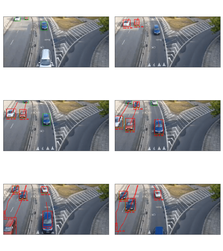
Running MultiTargetTracker example... Be patient...
Frame: 10/60
Frame: 20/60
Frame: 30/60
Frame: 40/60
Frame: 50/60
Frame: 60/60