Creating Smooth Transitions Between Coordinates

This is a demonstration of the get_smooth_transition_models() method for use with the MultiTransitionMovingPlatform.

This method takes a series of 2D cartesian coordinates, and returns a chain (list) of ConstantTurn transition models, alongside a list of transition times that each respective model should be used for.

Where required, the method also appends intermediate, custom, linear acceleration transition models Point2PointConstantAcceleration which accelerate (/decelerate) the platform to an appropriate speed whereby it arrives at the next destination coordinates on-time, or allows it to arrive before-hand, whereby it stops at the destination until the designated time (using the Point2PointStop custom transition model).

The method chooses the least change in bearing (\(b\)). Therefore altering its turn-rate (\(w\)) such that it turns left if its target destination is to its left (\(b\in [0, 180) \Rightarrow w > 0\)), and right if its destination is to the right (\(b\in (-180, 0) \Rightarrow w < 0\)).

Simple demonstration

Start with the target (platform) facing top-right (45 degrees clockwise from North). The target begins at the origin, at time = start.

Expect the target to make a sharp, left-turn to get on a course toward the second coordinate at (-10, 10).

import numpy as np
from datetime import timedelta, datetime
from matplotlib import pyplot as plt

start = datetime.now()

X = Y = np.array([0, -10, -20])
Y = np.array([0, 10, 0])
times = [start, start+timedelta(seconds=10), start+timedelta(seconds=30)]

Plotting the three target destinations (in blue) and the target initial bearing in green:

from stonesoup.types.array import StateVector
from stonesoup.types.state import State

ux = 1  # initial x-speed
uy = 1  # initial y-speed
platform_state = State(StateVector((X[0], ux, Y[0], uy)), timestamp=start)

fig = plt.figure(figsize=(10, 6))
ax = fig.add_subplot(1, 1, 1)
ax.set_xlabel("$x$")
ax.set_ylabel("$y$")
ax.axis('equal')
ax.scatter(X, Y, color='lightskyblue', s=100, edgecolors='black')
ax.plot((X[0], X[0] + 2*ux), (Y[0], Y[0] + 2*uy), color='lightgreen', linewidth=2)

Out:

[<matplotlib.lines.Line2D object at 0x7fc0ee429950>]

get_smooth_transition_models() requires the initial state of the platform, x and y coordinates, times to be at each respective coordinate and the platform turn-rate.

The ‘times’ parameter will dictate the times at which the target should be at each respective target coordinate. Hence, the first coordinate transition should take 10 seconds. The target starts off with insufficient speed, so we expect it to accelerate once out of the turn so as to get to the destination in a total of 10 seconds.

The target will have a constant turn rate of 25 degrees per second - a sharp turn, partly to guarantee that it can reach its destination in time, but also as initial velocity and angle turn-rate are constrained according to the following formulae (derived for the case where turn-rate (\(w\)) and initial bearing (\(a\)) are positive and \(< 180\) degrees):

where we must have that \(c \leq \frac{d\sin(b)}{\sin(wt)}\). Ie. the turn must be completed without the target ‘over-shooting’ the destination. Along with the constraint that the turn must be possible - if the turn-rate is too low, the target may never turn enough to hit the destination.

from stonesoup.simulator.transition import create_smooth_transition_models
transition_models, transition_times = create_smooth_transition_models(initial_state=platform_state,
                                                                      x_coords=X,
                                                                      y_coords=Y,
                                                                      times=times,
                                                                      turn_rate=np.radians(25))

This gives the transition times/models:

from stonesoup.models.transition.linear import ConstantTurn
for transition_time, transition_model in zip(transition_times, transition_models):
    print('Duration: ', transition_time.total_seconds(), 's ',
          'Model: ', type(transition_model), end=' ')
    if isinstance(transition_model, ConstantTurn):
        print('turn-rate: ', transition_model.turn_rate)
    else:
        print('x-acceleration: ', transition_model.ax, end=', ')
        print('y-acceleration: ', transition_model.ay)

Out:

Duration:  4.29188 s  Model:  <class 'stonesoup.models.transition.linear.ConstantTurn'> turn-rate:  0.4363323129985824
Duration:  5.70812 s  Model:  <class 'stonesoup.simulator.transition.Point2PointConstantAcceleration'> x-acceleration:  -0.12692604565249116, y-acceleration:  0.06664606400905905
Duration:  3.856929 s  Model:  <class 'stonesoup.models.transition.linear.ConstantTurn'> turn-rate:  0.4363323129985824
Duration:  16.143071 s  Model:  <class 'stonesoup.simulator.transition.Point2PointStop'> x-acceleration:  0.11502454961364292, y-acceleration:  0.29533082096657887

The last transition model calls a Point2PointStop transition model to bring the target to a complete stop (as a linear acceleration model would require the target to over-shoot the destination and turn-back on itself in order to arrive at the correct time).

Create a MultiTransitionMovingPlatform using the output transition models and times.

from stonesoup.platform.base import MultiTransitionMovingPlatform
platform = MultiTransitionMovingPlatform(states=platform_state,
                                         position_mapping=(0, 2),
                                         transition_models=transition_models,
                                         transition_times=transition_times)

Plot the platform path (light blue). Acceleration is shown by (dark blue) marker density (further apart => faster). The deceleration to 0-velocity at the 3rd target coordinate is clear. (Platform may be slightly off as transition times are rounded down).

platform_coords = []
for i in range(int((times[-1] - times[0]).total_seconds())):
    platform_coords.append((platform.state.state_vector[0], platform.state.state_vector[2]))
    platform.move(timestamp=start+timedelta(seconds=i))

ax.plot([coord[0] for coord in platform_coords],
        [coord[1] for coord in platform_coords],
        color='lightskyblue',
        marker='.',
        markerfacecolor='blue',
        linewidth=3)
fig

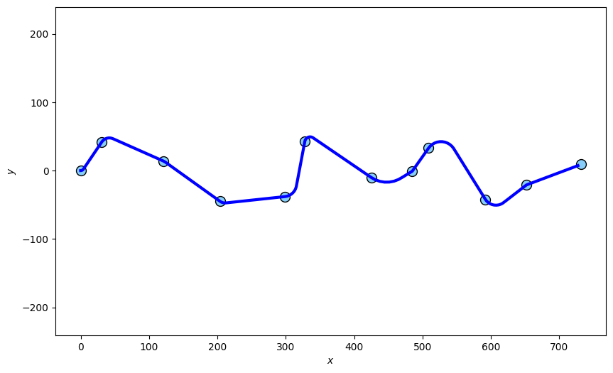
Running through multiple coordinates

A demonstration using several coordinates.

np.random.seed(101)

# Move in positive x-direction.
X = np.array([0])
for i in range(11):
    X = np.append(X, X[-1] + np.random.randint(20, 100))
print('X = ', X)

# Vary y in [-5, 5).
Y = np.array([0])
for i in range(11):
    Y = np.append(Y, np.random.randint(-50, 50))
print('Y = ', Y)

# 1 hour to get to each coord.
times = [start+timedelta(seconds=3600*i) for i in range(len(X))]  # Total of 12 hours

fig = plt.figure(figsize=(10, 6))
ax = fig.add_subplot(1, 1, 1)
ax.set_xlabel("$x$")
ax.set_ylabel("$y$")
ax.axis('equal')
ax.scatter(X, Y, color='lightskyblue', s=100, edgecolors='black')

Out:

X =  [  0  31 121 204 299 328 425 485 509 592 652 732]
Y =  [  0  42  14 -45 -38  43 -10  -1  33 -42 -21   9]

<matplotlib.collections.PathCollection object at 0x7fc0f1dc2790>

initial_vx = (X[1]-X[0]) / 3600  # initial x-speed
initial_vy = 0  # initial y-speed
platform_state = State((X[0], initial_vx, Y[0], initial_vy), timestamp=start)

transition_models, transition_times = create_smooth_transition_models(initial_state=platform_state,
                                                                      x_coords=X,
                                                                      y_coords=Y,
                                                                      times=times,
                                                                      turn_rate=np.radians(0.1))
platform = MultiTransitionMovingPlatform(states=platform_state,
                                         position_mapping=(0, 2),
                                         transition_models=transition_models,
                                         transition_times=transition_times)

platform_coords = []
sim_rate = 100  # 'sim_rate'-seconds each time-step.
for i in range(int((times[-1] - times[0]).total_seconds()/sim_rate)):
    platform_coords.append((platform.state.state_vector[0], platform.state.state_vector[2]))
    platform.move(timestamp=start+timedelta(seconds=sim_rate*i))
platform_coords.append((platform.state.state_vector[0], platform.state.state_vector[2]))

ax.plot([coord[0] for coord in platform_coords],
        [coord[1] for coord in platform_coords],
        color='blue',
        linewidth=3)
fig