Areas of interest based Reward Function

This notebook introduces sensor management which factors in environmental information related to the location the sensor is operating in.

We use the AreaOfInterest object, which has functionality for setting levels of “interest” within defined x, y boundaries, and the AOIAccessRewardFunction to define different behaviour for the sensor platform by switching between different reward functions.

Here we will define three areas with different levels of interest, to simulate a scenario where the sensor platform gets closer to the target to make observations as the target moves into a higher interest area.

Setting Up the Scenario

First we generate a ground truth of a target following a constant velocity with some noise and plot this.

import numpy as np
from datetime import datetime, timedelta


from stonesoup.models.transition.linear import (CombinedLinearGaussianTransitionModel,
                                                ConstantVelocity)
from stonesoup.types.groundtruth import GroundTruthPath, GroundTruthState

np.random.seed(1990)

start_time = datetime.now().replace(second=0, microsecond=0)

transition_model = CombinedLinearGaussianTransitionModel(
    [ConstantVelocity(10), ConstantVelocity(10)])

truths = []
truth = GroundTruthPath([GroundTruthState([-450, 5, 450, -5], timestamp=start_time)])
duration = 120
timesteps = [start_time]

for k in range(1, duration):
    timesteps.append(start_time+timedelta(seconds=k))
    truth.append(GroundTruthState(
        transition_model.function(truth[k-1], noise=True, time_interval=timedelta(seconds=1)),
        timestamp=timesteps[k]))
truths.append(truth)

from stonesoup.plotter import AnimatedPlotterly
plotter = AnimatedPlotterly(timesteps, tail_length=1)
plotter.plot_ground_truths(truth, [0, 2])
plotter.fig

Creating the Platform and Sensor

Next we create the taskable sensor platform and attach a RadarRotatingBearingRange sensor. We also create a target sensor, for the purpose of modelling the target’s field of view, for use in the FOVInteractionRewardFunction.

from stonesoup.platform import MovingPlatform
from stonesoup.movable.max_speed import MaxSpeedActionableMovable
from stonesoup.sensor.radar.radar import RadarRotatingBearingRange
from stonesoup.types.angle import Angle
from stonesoup.types.state import State, StateVector

sensor = RadarRotatingBearingRange(
    position_mapping=(0, 2),
    noise_covar=np.array([[np.radians(5)**2, 0],
                          [0, 20**2]]),
    ndim_state=4,
    rpm=30,
    fov_angle=np.radians(360),
    dwell_centre=StateVector([np.radians(0)]),
    max_range=300,

    resolution=Angle(np.radians(360)))

target_sensor = RadarRotatingBearingRange(
    position_mapping=(0, 2),
    noise_covar=np.array([[np.radians(1)**2, 0], [0, 1**2]]),
    ndim_state=4,
    rpm=30,
    fov_angle=np.radians(360),
    dwell_centre=StateVector([np.radians(90)]),
    max_range=100,
    resolution=Angle(np.radians(180)))

platform = MovingPlatform(
    movement_controller=MaxSpeedActionableMovable(
        states=[State([-500, 700],
                      timestamp=start_time)],
        position_mapping=(0, 1),
        action_mapping=(0, 1),
        resolution=10,
        angle_resolution=np.pi/2,
        max_speed=100),
    sensors=[sensor])

Creating a Predictor and Updater

Next we need some tracking components: a predictor and an updater.

from stonesoup.predictor.kalman import KalmanPredictor
predictor = KalmanPredictor(transition_model)

from stonesoup.updater.kalman import ExtendedKalmanUpdater
updater = ExtendedKalmanUpdater(measurement_model=None)

Creating Areas of Interest

Different areas of interest can be defined by setting minimum/maximum values for x and y using the AreaOfInterest. Here we have 3 areas of different levels of interest.

Area 1 is defined as being everything to the left of the origin (x = 0), with an interest level of 4. Area 2 is defined as being between x = 0 and x = 1500, with an interest level of 7. Area 3 is defined as being everything to the right of x = 1500, with an interest level of 10.

from stonesoup.types.shape import AreaOfInterest

area1 = AreaOfInterest(xmax=0, interest=4)
area2 = AreaOfInterest(xmin=0, xmax=1500, interest=7)
area3 = AreaOfInterest(xmin=1500, interest=10)

Creating a Sensor Manager

Now we create a sensor manager, providing it with the sensor, the sensor platform, and a reward function.

We define a different reward function for each area of interest. In areas of low interest we use a combination of the FOVInteractionRewardFunction and the UncertaintyRewardFunction, ensuring the sensor platform stays outside a set distance from the target while continuing to track it. In areas of medium interest this distance is reduced, and in areas of high interest the FOVInteractionRewardFunction is not used, so the sensor platform can get as close as it likes.

The AOIAccessRewardFunction is used to switch between these reward functions as the target moves through the different areas of interest, based on the target’s location and the defined interest thresholds for each area.

from stonesoup.sensormanager.reward import (
    UncertaintyRewardFunction, MultiplicativeRewardFunction, FOVInteractionRewardFunction,
    AOIRewardFunction2D)

from stonesoup.sensormanager.base import BruteForceSensorManager

reward_func_A = UncertaintyRewardFunction(predictor, updater)

reward_func_B = FOVInteractionRewardFunction(
    predictor, updater, sensor_fov_radius=sensor.max_range,
    target_fov_radius=target_sensor.max_range + 100,
    fov_scale=1)

reward_func_C = FOVInteractionRewardFunction(
    predictor, updater, sensor_fov_radius=sensor.max_range,
    target_fov_radius=target_sensor.max_range,
    fov_scale=0.75)

reward_func_AB = MultiplicativeRewardFunction([reward_func_A, reward_func_B])
reward_func_AC = MultiplicativeRewardFunction([reward_func_A, reward_func_C])


reward_func_aoi = AOIRewardFunction2D(default_reward=reward_func_AC,
                                            interest_thresholds={3: reward_func_AB,
                                                                 5: reward_func_AC,
                                                                 9: reward_func_A},
                                            areas=[area1, area2, area3],
                                            target_mapping=[0, 2])

sensormanager = BruteForceSensorManager(sensors={sensor},
                                        platforms={platform},
                                        reward_function=reward_func_aoi,)

Creating a Tracker

Next we initialise a track and build a tracker.

from stonesoup.types.state import GaussianState
from stonesoup.types.track import Track

prior = GaussianState(truths[0][0].state_vector,
                      covar=np.diag([0.5, 0.5, 0.5, 0.5] + np.random.normal(0, 5e-4, 4)),
                      timestamp=start_time)

tracks = {Track([prior])}

from stonesoup.hypothesiser.distance import DistanceHypothesiser
from stonesoup.measures import Mahalanobis

hypothesiser = DistanceHypothesiser(predictor, updater, measure=Mahalanobis(), missed_distance=5)

from stonesoup.dataassociator.neighbour import GNNWith2DAssignment
data_associator = GNNWith2DAssignment(hypothesiser)

Running the Tracking Loop

At each timestep the sensor manager generates the optimal actions for our sensor and platform. These actions are taken before the sensor makes detections and the track is updated.

from ordered_set import OrderedSet
from collections import defaultdict
import copy
from stonesoup.measures import Euclidean
from stonesoup.sensor.sensor import Sensor

all_measurements = set()
sensor_history = defaultdict(dict)
for timestep in timesteps[1:]:

    chosen_actions = sensormanager.choose_actions(tracks, timestep)
    measurements = set()

    for chosen_action in chosen_actions:
        for actionable, actions in chosen_action.items():
            actionable.add_actions(actions)
            actionable.act(timestep)
            if isinstance(actionable, Sensor):
                measurements |= actionable.measure(OrderedSet(truth[timestep] for truth in truths),
                                                   noise=True)

    all_measurements.update(measurements)
    sensor_history[timestep][sensor] = copy.deepcopy(sensor)
    hypotheses = data_associator.associate(tracks, measurements, timestep)
    for track in tracks:
        hypothesis = hypotheses[track]
        if hypothesis.measurement:
            post = updater.update(hypothesis)
            track.append(post)
        else:
            track.append(hypothesis.prediction)

Plotting

Now we use the animated plotter to see what behaviour has been achieved.

import plotly.graph_objects as go
from stonesoup.platform.base import PathBasedPlatform

plotter = AnimatedPlotterly(timesteps, tail_length=0.1)
plotter.plot_ground_truths(truths, [0, 2], mode='lines', line=dict(dash=None))
plotter.plot_tracks(tracks, mapping=(0, 2))
plotter.plot_measurements(all_measurements, mapping=(0, 2))

track_list = list(tracks)
target_platform = PathBasedPlatform(path=track_list[0], sensors=[target_sensor],
                                    position_mapping=[0, 2])
target_sensor_history = defaultdict(dict)

for timestep in timesteps[1:]:
    target_platform.move(timestep)
    target_sensor_history[timestep][target_sensor] = copy.deepcopy(target_sensor)
target_sensor_set = {target_sensor}
sensor_set = {sensor}

plotter.plot_sensor_fov(sensor_set, sensor_history)

plotter.plot_sensor_fov(target_sensor_set, target_sensor_history, label="Target FOV", colour="red")
plotter.fig.add_trace(go.Scatter(x=[1500, 1500], y=[-300, 500], mode='lines',
                                 line=dict(color='#888'),
                                 name='Area Boundaries',
                                 showlegend=False))
plotter.fig.add_trace(go.Scatter(x=[0, 0], y=[-300, 500], mode='lines',
                                 line=dict(color='#888'),
                                 name='Area Boundaries',
                                 showlegend=False))
plotter.fig.add_trace(go.Scatter(x=[-400, 800, 2000],
                                 y=[0, 0, 0], mode="text", name="Areas of Interest",
                                 line=dict(color='#888'),
                                 text=["Interest: 4",
                                       "Interest: 7",
                                       "Interest: 10"]))
plotter.fig

The actionable platform is able to follow the target as it moves across the action space, initially remaining outside the distance set for areas of low interest, then getting closer as it moves into areas of higher interest.

This is a relatively simple example but demonstrates how the sensor manager can switch reward function, and therefore change behaviour, based on information about its environment.

Metrics

To check the impact this has on the tracking performance we compute some metrics.

from stonesoup.metricgenerator.ospametric import OSPAMetric
ospa_generatorA = OSPAMetric(c=40, p=1,
                             generator_name='3 areas of interest',
                             tracks_key='tracksA',
                             truths_key='truths')

from stonesoup.metricgenerator.tracktotruthmetrics import SIAPMetrics
siap_generatorA = SIAPMetrics(position_measure=Euclidean((0, 2)),
                              velocity_measure=Euclidean((1, 3)),
                              generator_name='3 areas of interest',
                              tracks_key='tracksA',
                              truths_key='truths')

from stonesoup.dataassociator.tracktotrack import TrackToTruth
associator = TrackToTruth(association_threshold=30)

from stonesoup.metricgenerator.uncertaintymetric import SumofCovarianceNormsMetric
uncertainty_generatorA = SumofCovarianceNormsMetric(generator_name='3 areas of interest',
                                                    tracks_key='tracksA')

from stonesoup.metricgenerator.manager import MultiManager

metric_manager = MultiManager([ospa_generatorA,
                               siap_generatorA,
                               uncertainty_generatorA],
                              associator=associator)

metric_manager.add_data({'truths': truths, 'tracksA': tracks})

metrics = metric_manager.generate_metrics()

First we plot Sum of Covariance Norms metric.

from stonesoup.plotter import MetricPlotter

fig1 = MetricPlotter()
fig1.plot_metrics(metrics, metric_names=['Sum of Covariance Norms Metric'])

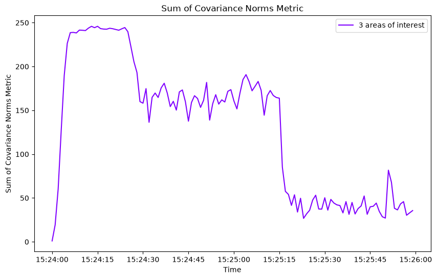
We can see from this that initially, when the sensor platform is staying further from the target, the track uncertainty is higher, and as it moves into an area of high interest, it gets closer to the target and the track uncertainty reduces.

Next we plot the OSPA and SIAP metrics

fig2 = MetricPlotter()
fig2.plot_metrics(metrics, metric_names=['OSPA distances'])

fig3 = MetricPlotter()
fig3.plot_metrics(metrics, metric_names=['SIAP Position Accuracy at times',
                                         'SIAP Velocity Accuracy at times'])

• 
• 

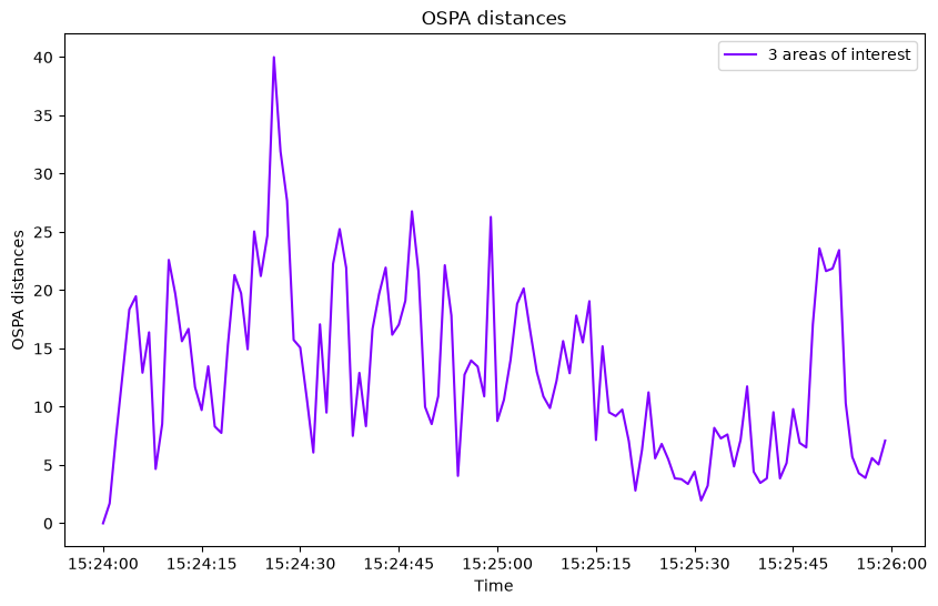
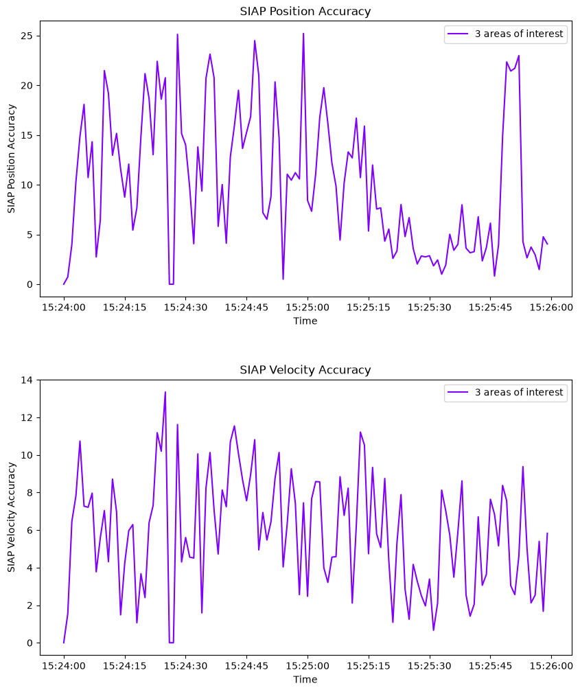
These metrics show a similar tracking performance across the simulation, even where track uncertainty is greater.