1 - An introduction to Stone Soup: using the Kalman filter

This notebook is designed to introduce some of the basic features of Stone Soup using a single target scenario and a Kalman filter as an example.

Background and notation

Let \(p(\mathbf{x}_{k})\), the probability distribution over \(\mathbf{x}_{k} \in \mathbb{R}^n\), represent a hidden state at some discrete point \(k\). The \(k\) is most often interpreted as a timestep, but could be any sequential index (hence we don’t use \(t\)). The measurement is given by \(\mathbf{z}_{k} \in \mathbb{R}^m\).

In Stone Soup, objects derived from the State class carry information on a variety of states, whether they be hidden states, observations, ground truth. Minimally, a state will comprise a StateVector and a timestamp. These can be extended. For example the GaussianState is parameterised by a mean state vector and a covariance matrix. (We’ll see this in action later.)

Our goal is to infer \(p(\mathbf{x}_{k})\), given a sequence of measurements \(\mathbf{z}_{1}, ..., \mathbf{z}_{k}\), (which we’ll write as \(\mathbf{z}_{1:k}\)). In general \(\mathbf{z}\) can include clutter and false alarms. We’ll defer those complications to later tutorials and assume, for the moment, that all measurements are generated by a target, and that detecting the target at each timestep is certain (\(p_d = 1\) and \(p_{fa} = 0\)).

Prediction

We proceed under the Markovian assumption that \(p(\mathbf{x}_k) = \int_{-\infty} ^{\infty} p(\mathbf{x}_k|\mathbf{x}_{k-1}) p(\mathbf{x}_{k-1}) d \mathbf{x}_{k-1}\), meaning that the distribution over the state of an object at time \(k\) can be predicted entirely from its state at previous time \(k-1\). If our understanding of \(p(\mathbf{x}_{k-1})\) was informed by a series of measurements up to and including timestep \(k-1\), we can write

\[p(\mathbf{x}_k|\mathbf{z}_{1:k-1}) = \int_{-\infty}^{\infty} p(\mathbf{x}_k|\mathbf{x}_{k-1}) p(\mathbf{x}_{k-1}|\mathbf{z}_{1:k-1})d \mathbf{x}_{k-1}\]

This is known as the Chapman-Kolmogorov equation. In Stone Soup we refer to this process as prediction and to an object that undertakes it as a Predictor. A predictor requires a state transition model, namely a function which undertakes \(\mathbf{x}_{k|k-1} = f(\mathbf{x}_{k-1}, \mathbf{w}_k)\), where \(\mathbf{w}_k\) is a noise term. Stone Soup has transition models derived from the TransitionModel class.

Update

We assume a sensor measurement is generated by some stochastic process represented by a function, \(\mathbf{z}_k = h(\mathbf{x}_k, \boldsymbol{\nu}_k)\) where \(\boldsymbol{\nu}_k\) is the noise.

The goal of the update process is to generate the posterior state estimate, from the prediction and the measurement. It does this by way of Bayes’ rule,

\[p(\mathbf{x}_k | \mathbf{z}_{1:k}) = \frac{ p(\mathbf{z}_{k} | \mathbf{x}_k) p(\mathbf{x}_k | \mathbf{z}_{1:k-1})} {p(\mathbf{z}_k)}\]

where \(p(\mathbf{x}_k | \mathbf{z}_{1:k-1})\) is the output of the prediction stage, \(p(\mathbf{z}_{k} | \mathbf{x}_k)\) is known as the likelihood, and \(p(\mathbf{z}_k)\) the evidence. In Stone Soup, this calculation is undertaken by the Updater class. Updaters use a MeasurementModel class which models the effect of \(h(\cdot)\).

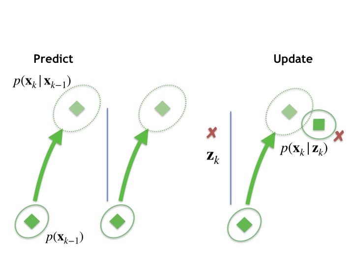
This figure represents a single instance of this predict-update process. It shows a prior distribution, at the bottom left, a prediction (dotted ellipse), and posterior (top right) calculated after a measurement update. We then proceed recursively, the posterior distribution at \(k\) becoming the prior for the next measurement timestep, and so on.

A nearly-constant velocity example

We’re going to set up a simple scenario in which a target moves at constant velocity with the addition of some random noise, (referred to as a nearly constant velocity model).

As is customary in Python scripts we begin with some imports. (These ones allow us access to mathematical and timing functions.)

import numpy as np
from datetime import datetime, timedelta

Simulate a target

We consider a 2d Cartesian scheme where the state vector is \([x \ \dot{x} \ y \ \dot{y}]^T\). That is, we’ll model the target motion as a position and velocity component in each dimension. The units used are unimportant, but do need to be consistent.

To start we’ll create a simple truth path, sampling at 1 second intervals. We’ll do this by employing one of Stone Soup’s native transition models.

These inputs are required:

from stonesoup.types.groundtruth import GroundTruthPath, GroundTruthState
from stonesoup.models.transition.linear import CombinedLinearGaussianTransitionModel, \
                                               ConstantVelocity

# And the clock starts
start_time = datetime.now()

We note that it can sometimes be useful to fix our random number generator in order to probe a particular example repeatedly.

np.random.seed(1991)

The ConstantVelocity class creates a one-dimensional constant velocity model with Gaussian noise. For this simulation \(\mathbf{x}_k = F_k \mathbf{x}_{k-1} + \mathbf{w}_k\), \(\mathbf{w}_k \sim \mathcal{N}(0,Q)\), with

\[\begin{split}F_{k} &= \begin{bmatrix} 1 & \triangle t \\ 0 & 1 \\ \end{bmatrix} \\ Q_k &= \begin{bmatrix} \frac{\triangle t^3}{3} & \frac{\triangle t^2}{2} \\ \frac{\triangle t^2}{2} & \triangle t \\ \end{bmatrix} q\end{split}\]

where \(q\), the input parameter to ConstantVelocity, is the magnitude of the noise per \(\triangle t\)-sized timestep.

The CombinedLinearGaussianTransitionModel class takes a number of 1d models and combines them in a linear Gaussian model of arbitrary dimension, \(D\).

\[\begin{split}F_{k}^{D} &= \begin{bmatrix} F_k^{1} & & \mathbf{0} \\ & \ddots & \\ \mathbf{0} & & F_k^d \\ \end{bmatrix}\\ Q_{k}^{D} &= \begin{bmatrix} Q_k^{1} & & \mathbf{0} \\ & \ddots & \\ \mathbf{0} & & Q_k^d \\ \end{bmatrix}\end{split}\]

We want a 2d simulation, so we’ll do:

q_x = 0.05
q_y = 0.05
transition_model = CombinedLinearGaussianTransitionModel([ConstantVelocity(q_x),
                                                          ConstantVelocity(q_y)])

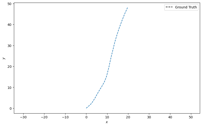
A ‘truth path’ is created starting at (0,0) moving to the NE at one distance unit per (time) step in each dimension.

truth = GroundTruthPath([GroundTruthState([0, 1, 0, 1], timestamp=start_time)])

num_steps = 20
for k in range(1, num_steps + 1):
    truth.append(GroundTruthState(
        transition_model.function(truth[k-1], noise=True, time_interval=timedelta(seconds=1)),
        timestamp=start_time+timedelta(seconds=k)))

Thus the ground truth is generated and we can plot the result.

Stone Soup has an in-built plotting class which can be used to plot ground truths, measurements and tracks in a consistent format. It can be accessed by importing the class Plotter from Stone Soup as below.

Note that the mapping argument is [0, 2] because those are the x and y position indices from our state vector.

from stonesoup.plotter import Plotter
plotter = Plotter()
plotter.plot_ground_truths(truth, [0, 2])

We can check the \(F_k\) and \(Q_k\) matrices (generated over a 1s period).

transition_model.matrix(time_interval=timedelta(seconds=1))

Out:

array([[1., 1., 0., 0.],
       [0., 1., 0., 0.],
       [0., 0., 1., 1.],
       [0., 0., 0., 1.]])

transition_model.covar(time_interval=timedelta(seconds=1))

Out:

array([[0.01666667, 0.025     , 0.        , 0.        ],
       [0.025     , 0.05      , 0.        , 0.        ],
       [0.        , 0.        , 0.01666667, 0.025     ],
       [0.        , 0.        , 0.025     , 0.05      ]])

At this point you can play with the various parameters and see how it affects the simulated output.

Simulate measurements

We’ll use one of Stone Soup’s measurement models in order to generate measurements from the ground truth. For the moment we assume a ‘linear’ sensor which detects the position, but not velocity, of a target, such that \(\mathbf{z}_k = H_k \mathbf{x}_k + \boldsymbol{\nu}_k\), \(\boldsymbol{\nu}_k \sim \mathcal{N}(0,R)\), with

\[\begin{split}H_k &= \begin{bmatrix} 1 & 0 & 0 & 0\\ 0 & 0 & 1 & 0\\ \end{bmatrix}\\ R &= \begin{bmatrix} 1 & 0\\ 0 & 1\\ \end{bmatrix} \omega\end{split}\]

where \(\omega\) is set to 5 initially (but again, feel free to play around).

We’re going to need a Detection type to store the detections, and a LinearGaussian measurement model.

from stonesoup.types.detection import Detection
from stonesoup.models.measurement.linear import LinearGaussian

The linear Gaussian measurement model is set up by indicating the number of dimensions in the state vector and the dimensions that are measured (so specifying \(H_k\)) and the noise covariance matrix \(R\).

measurement_model = LinearGaussian(
    ndim_state=4,  # Number of state dimensions (position and velocity in 2D)
    mapping=(0, 2),  # Mapping measurement vector index to state index
    noise_covar=np.array([[5, 0],  # Covariance matrix for Gaussian PDF
                          [0, 5]])
    )

Check the output is as we expect

measurement_model.matrix()

Out:

array([[1., 0., 0., 0.],
       [0., 0., 1., 0.]])

measurement_model.covar()

Out:

array([[5, 0],
       [0, 5]])

Generate the measurements

measurements = []
for state in truth:
    measurement = measurement_model.function(state, noise=True)
    measurements.append(Detection(measurement,
                                  timestamp=state.timestamp,
                                  measurement_model=measurement_model))

Plot the result, again mapping the x and y position values

plotter.plot_measurements(measurements, [0, 2])
plotter.fig

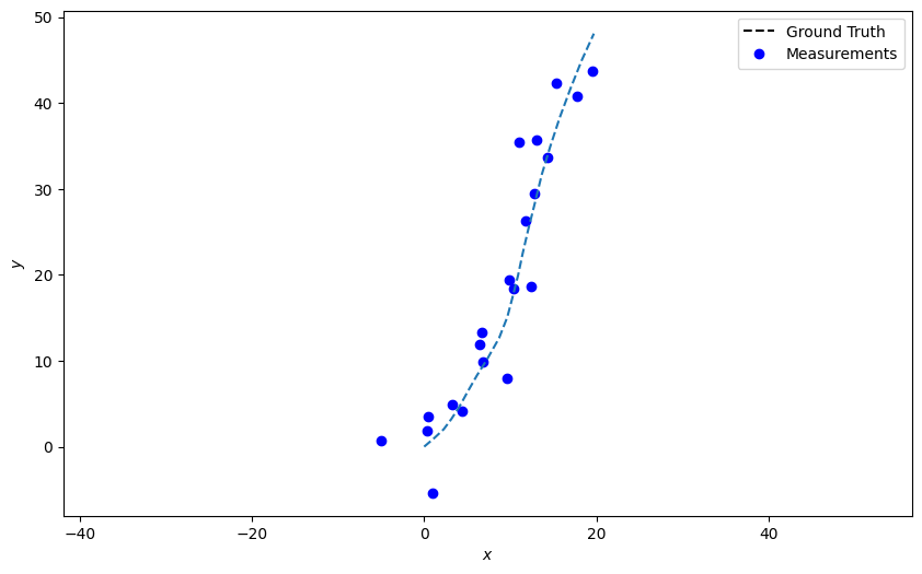
At this stage you should have a moderately linear ground truth path (dotted line) with a series of simulated measurements overplotted (blue circles). Take a moment to fiddle with the numbers in \(Q\) and \(R\) to see what it does to the path and measurements.

Construct a Kalman filter

We’re now ready to build a tracker. We’ll use a Kalman filter as it’s conceptually the simplest to start with. The Kalman filter is described extensively elsewhere 1, 2, so for the moment we just assert that the prediction step proceeds as:

\[\begin{split}\mathbf{x}_{k|k-1} &= F_{k}\mathbf{x}_{k-1} + B_{k}\mathbf{u}_{k}\\ P_{k|k-1} &= F_{k}P_{k-1}F_{k}^T + Q_{k},\end{split}\]

\(B_k \mathbf{u}_k\) is a control term which we’ll ignore for now (we assume we don’t influence the target directly).

The update step is:

\[\begin{split}\mathbf{x}_{k} &= \mathbf{x}_{k|k-1} + K_k(\mathbf{z}_k - H_{k}\mathbf{x}_{k|k-1})\\ P_{k} &= P_{k|k-1} - K_k H_{k} P_{k|k-1}\\\end{split}\]

where,

\[\begin{split}K_k &= P_{k|k-1} H_{k}^T S_k^{-1}\\ S_k &= H_{k} P_{k|k-1} H_{k}^T + R_{k}\end{split}\]

\(\mathbf{z}_k - H_{k}\mathbf{x}_{k|k-1}\) is known as the innovation and \(S_k\) the innovation covariance; \(K_k\) is the Kalman gain.

Constructing a predictor and updater in Stone Soup is simple. In a nice division of responsibility, a Predictor takes a TransitionModel as input and an Updater takes a MeasurementModel as input. Note that for now we’re using the same models used to generate the ground truth and the simulated measurements. This won’t usually be possible and it’s an interesting exercise to explore what happens when these parameters are mismatched.

from stonesoup.predictor.kalman import KalmanPredictor
predictor = KalmanPredictor(transition_model)

from stonesoup.updater.kalman import KalmanUpdater
updater = KalmanUpdater(measurement_model)

Run the Kalman filter

Now we have the components, we can execute the Kalman filter estimator on the simulated data.

In order to start, we’ll need to create the first prior estimate. We’re going to use the GaussianState we mentioned earlier. As the name suggests, this parameterises the state as \(\mathcal{N}(\mathbf{x}_0, P_0)\). By happy chance the initial values are chosen to match the truth quite well. You might want to manipulate these to see what happens.

from stonesoup.types.state import GaussianState
prior = GaussianState([[0], [1], [0], [1]], np.diag([1.5, 0.5, 1.5, 0.5]), timestamp=start_time)

In this instance data association is done somewhat implicitly. There is one prediction and one detection per timestep so no need to think too deeply. Stone Soup discourages such (undesirable) practice and requires that a Prediction and Detection are associated explicitly. This is done by way of a Hypothesis; the most simple is a SingleHypothesis which associates a single predicted state with a single detection. There is much more detail on how the Hypothesis class is used in later tutorials.

from stonesoup.types.hypothesis import SingleHypothesis

With this, we’ll now loop through our measurements, predicting and updating at each timestep. Uncontroversially, a Predictor has predict() function and an Updater an update() to do this. Storing the information is facilitated by the top-level Track class which holds a sequence of states.

from stonesoup.types.track import Track
track = Track()
for measurement in measurements:
    prediction = predictor.predict(prior, timestamp=measurement.timestamp)
    hypothesis = SingleHypothesis(prediction, measurement)  # Group a prediction and measurement
    post = updater.update(hypothesis)
    track.append(post)
    prior = track[-1]

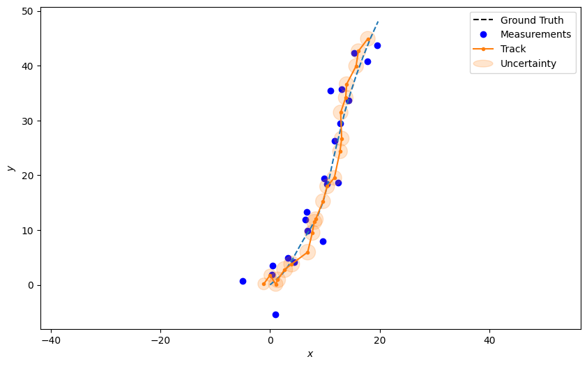
Plot the resulting track, including uncertainty ellipses

plotter.plot_tracks(track, [0, 2], uncertainty=True)
plotter.fig

Key points

1. Stone Soup is built on a variety of types of State object. These can be used to represent hidden states, observations, estimates, ground truth, and more.

2. Bayesian recursion is undertaken by the successive applications of predict and update methods using a Predictor and an Updater. Explicit association of predicted states with measurements is necessary. Broadly speaking, predictors apply a TransitionModel, data associators use a Hypothesiser to associate a prediction with a measurement, and updaters use this association together with the MeasurementModel to calculate the posterior state estimate.

References

1

Kalman 1960, A New Approach to Linear Filtering and Prediction Problems, Transactions of the ASME, Journal of Basic Engineering, 82 (series D), 35 (https://pdfs.semanticscholar.org/bb55/c1c619c30f939fc792b049172926a4a0c0f7.pdf?_ga=2.51363242.2056055521.1592932441-1812916183.1592932441)

2

Anderson & Moore 1979, Optimal filtering, (http://users.cecs.anu.edu.au/~john/papers/BOOK/B02.PDF)