Note
Click here to download the full example code or to run this example in your browser via Binder
6 - Data association - multi-target tracking tutorial
Tracking multiple targets through clutter
As we’ve seen, more often than not, the difficult part of state estimation concerns the ambiguous association of predicted states with measurements. This happens whenever there is more that one target under consideration, there are false alarms or clutter, targets can appear and disappear. That is to say it happens everywhere.
In this tutorial we introduce global nearest neighbour data association, which attempts to find a globally-consistent collection of hypotheses such that some overall score of correct association is maximised.
Background
Make the assumption that each target generates, at most, one measurement, and that one measurement is generated by, at most, a single target, or is a clutter point. Under these assumptions, global nearest neighbour will assign measurements to predicted measurements to minimise a total (global) cost which is a function of the sum of innovations. This is an example of an assignment problem in combinatorial optimisation.
With multiple targets to track, the NearestNeighbour algorithm compiles a list of all
hypotheses and selects pairings with higher scores first.
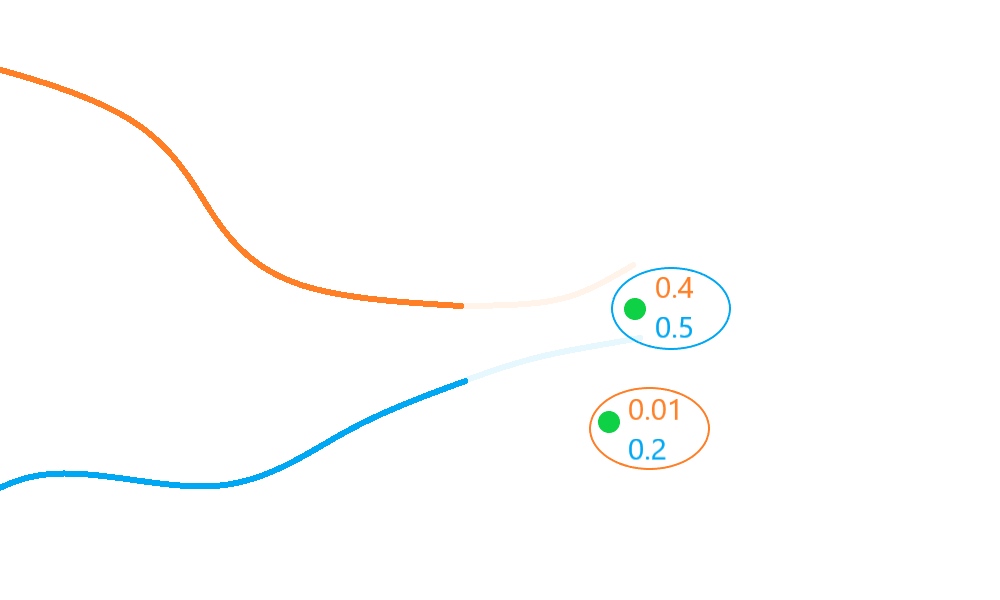
In the diagram above, the top detection is selected for association with the blue track, as this has the highest score/probability (\(0.5\)), and (as each measurement is associated at most once) the remaining detection must then be associated with the orange track, giving a net global score/probability of \(0.51\).
The GlobalNearestNeighbour evaluates all valid (distance-based) hypotheses
(measurement-prediction pairs) and selects the subset with the
greatest net ‘score’ (the collection of hypotheses pairs which have a minimum sum of distances
overall).
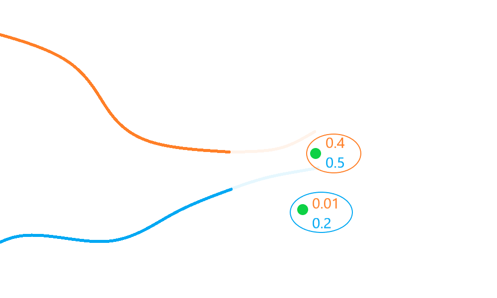
In the diagram above, the blue track is associated to the bottom detection even though the top detection scores higher relative to it. This association leads to a global score/probability of \(0.6\) - a better net score/probability than the \(0.51\) returned by the nearest neighbour algorithm.
A multi-target simulation
We start by simulating 2 targets moving in different directions across the 2D Cartesian plane. They start at (0, 0) and (0, 20) and cross roughly half-way through their transit.
import numpy as np
from datetime import datetime, timedelta
start_time = datetime.now()

from stonesoup.models.transition.linear import CombinedLinearGaussianTransitionModel, \
                                               ConstantVelocity
from stonesoup.types.groundtruth import GroundTruthPath, GroundTruthState
Generate ground truth
np.random.seed(1991)

truths = set()

transition_model = CombinedLinearGaussianTransitionModel([ConstantVelocity(0.005),
                                                          ConstantVelocity(0.005)])

truth = GroundTruthPath([GroundTruthState([0, 1, 0, 1], timestamp=start_time)])
for k in range(1, 21):
    truth.append(GroundTruthState(
        transition_model.function(truth[k-1], noise=True, time_interval=timedelta(seconds=1)),
        timestamp=start_time+timedelta(seconds=k)))
truths.add(truth)

truth = GroundTruthPath([GroundTruthState([0, 1, 20, -1], timestamp=start_time)])
for k in range(1, 21):
    truth.append(GroundTruthState(
        transition_model.function(truth[k-1], noise=True, time_interval=timedelta(seconds=1)),
        timestamp=start_time+timedelta(seconds=k)))
truths.add(truth)
Plot the ground truth
from stonesoup.plotter import Plotter
plotter = Plotter()
plotter.ax.set_ylim(0, 25)
plotter.plot_ground_truths(truths, [0, 2])

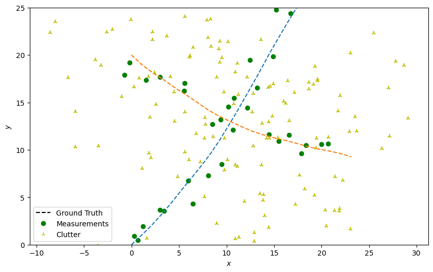
Generate detections with clutter
Next, generate detections with clutter just as in the previous tutorial. This time, we generate clutter about each state at each time-step.
from scipy.stats import uniform

from stonesoup.types.detection import TrueDetection
from stonesoup.types.detection import Clutter
from stonesoup.models.measurement.linear import LinearGaussian

measurement_model = LinearGaussian(
    ndim_state=4,
    mapping=(0, 2),
    noise_covar=np.array([[0.75, 0],
                          [0, 0.75]])
    )
all_measurements = []

for k in range(20):
    measurement_set = set()

    for truth in truths:
        # Generate actual detection from the state with a 10% chance that no detection is received.
        if np.random.rand() <= 0.9:
            measurement = measurement_model.function(truth[k], noise=True)
            measurement_set.add(TrueDetection(state_vector=measurement,
                                              groundtruth_path=truth,
                                              timestamp=truth[k].timestamp,
                                              measurement_model=measurement_model))

        # Generate clutter at this time-step
        truth_x = truth[k].state_vector[0]
        truth_y = truth[k].state_vector[2]
        for _ in range(np.random.randint(10)):
            x = uniform.rvs(truth_x - 10, 20)
            y = uniform.rvs(truth_y - 10, 20)
            measurement_set.add(Clutter(np.array([[x], [y]]), timestamp=truth[k].timestamp,
                                        measurement_model=measurement_model))
    all_measurements.append(measurement_set)

# Plot true detections and clutter.
plotter.plot_measurements(all_measurements, [0, 2], color='g')
plotter.fig
Create the Kalman predictor and updater
from stonesoup.predictor.kalman import KalmanPredictor
predictor = KalmanPredictor(transition_model)

from stonesoup.updater.kalman import KalmanUpdater
updater = KalmanUpdater(measurement_model)
As in the clutter tutorial, we will quantify predicted-measurement to measurement distance using the Mahalanobis distance.
from stonesoup.hypothesiser.distance import DistanceHypothesiser
from stonesoup.measures import Mahalanobis
hypothesiser = DistanceHypothesiser(predictor, updater, measure=Mahalanobis(), missed_distance=3)


from stonesoup.dataassociator.neighbour import GlobalNearestNeighbour
data_associator = GlobalNearestNeighbour(hypothesiser)
Run the Kalman filters
We create 2 priors reflecting the targets’ initial states.
from stonesoup.types.state import GaussianState
prior1 = GaussianState([[0], [1], [0], [1]], np.diag([1.5, 0.5, 1.5, 0.5]), timestamp=start_time)
prior2 = GaussianState([[0], [1], [20], [-1]], np.diag([1.5, 0.5, 1.5, 0.5]), timestamp=start_time)
Loop through the predict, hypothesise, associate and update steps.
from stonesoup.types.track import Track
tracks = {Track([prior1]), Track([prior2])}

for n, measurements in enumerate(all_measurements):
    # Calculate all hypothesis pairs and associate the elements in the best subset to the tracks.
    hypotheses = data_associator.associate(tracks,
                                           measurements,
                                           start_time + timedelta(seconds=n))
    for track in tracks:
        hypothesis = hypotheses[track]
        if hypothesis.measurement:
            post = updater.update(hypothesis)
            track.append(post)
        else:  # When data associator says no detections are good enough, we'll keep the prediction
            track.append(hypothesis.prediction)
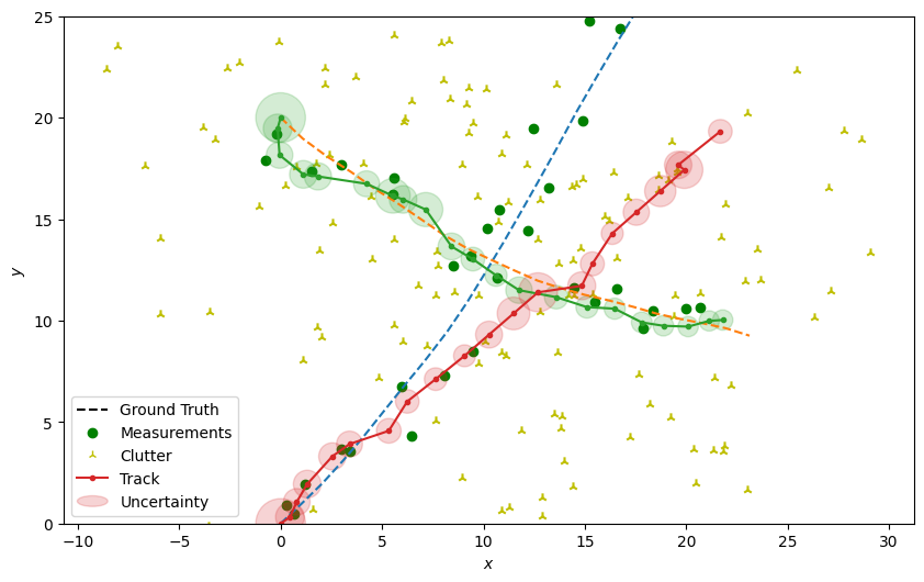
Plot the resulting tracks
plotter.plot_tracks(tracks, [0, 2], uncertainty=True)
plotter.fig
Total running time of the script: ( 0 minutes 1.821 seconds)