1 - Single Sensor Management

This tutorial introduces the sensor manager classes in Stone Soup which can be used to build simple sensor management algorithms for tracking and state estimation. The intention is to further build on these base classes to develop more complex sensor management algorithms.

Background

Sensor management is the process of deciding and executing the actions that a sensor, or group of sensors will take in a specific scenario and with a particular objective, or objectives in mind. The process involves using information about the scenario to determine an appropriate action for the sensing system to take. An observation of the state of the system is then made using the sensing configuration decided by the sensor manager. The observations are used to update the estimate of the collective states and this update is used (if necessary) to determine the next action for the sensing system to take.

A simple example can be imagined using a sensor with a limited field of view which must decide which direction it should point in at each time step. Alternatively, we might construct an objective based example by imagining that the desired target is fast moving and the sensor can only observe one target at a time. If there are multiple targets which could be observed the sensor manager could choose to observe the target that had the greatest estimated velocity at the current time.

The example in this notebook considers two simple sensor management methods and applies them to the same ground truths in order to quantify the difference in behaviour. The scenario simulates 3 targets moving on nearly constant velocity trajectories and a radar with a specified field of view, which can be pointed in a particular direction.

The first method, using the class RandomSensorManager chooses a direction to point in randomly with equal probability. The second method, using the class BruteForceSensorManager considers every possible direction the sensor could point in and uses a reward function to determine the best choice of action. In this example the reward function aims to reduce the total uncertainty of the track estimates at each time step. To achieve this the sensor manager chooses to look in the direction which results in the greatest reduction in uncertainty - as represented by the Frobenius norm of the covariance matrix.

Sensor management as a POMDP

Sensor management problems can be considered as Partially Observable Markov Decision Processes (POMDPs) where observations provide information about the current state of the system but there is uncertainty in the estimate of the underlying state due to noisy sensors and imprecise models of target evaluation.

POMDPs consist of:

• \(X_k\), the finite set of possible states for each stage index \(k\).

• \(A_k\), the finite set of possible actions for each stage index \(k\).

• \(R_k(x, a)\), the reward function.

• \(Z_k\), the finite set of possible observations for each stage index \(k\).

• \(f_k(x_{k}|x_{k-1})\), a (set of) state transition function(s). (Note that actions are excluded from the function at the moment. It may be necessary to include them if prior sensor actions cause the targets to modify their behaviour.)

• \(h_k(z_k | x_k, a_k)\), a (set of) observation function(s).

• \(\{x\}_k\), the set of states at \(k\) to be estimated.

• \(\{a\}_k\), a set of actions at \(k\) to be chosen.

• \(\{z\}_k\), the observations at \(k\) returned by the sensor.

• \(\Psi_{k-1}\), denotes the complete set of ‘intelligence’ available to the sensor manager before deciding on an action at \(k\). This includes the prior set of state estimates \(\{x\}_{k-1}\), but may also encompass contextual information, sensor constraints or mission parameters.

Figure 1: Illustration of sequential actions and measurements. [1]

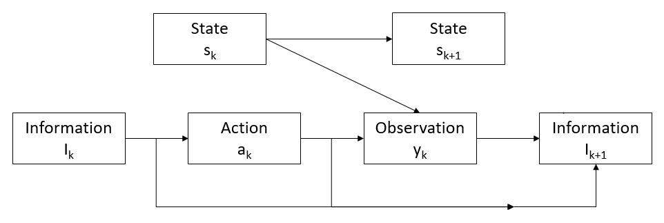
\(\Psi_k\) is the intelligence available to the sensor manager at stage index \(k\), to help select the action \(a_k\) for the system to take. An observation \(z_k\) is made by the sensing system, giving information on the state \(x_k\). The action \(a_k\) and observation \(z_k\) are added to the intelligence set to generate \(\Psi_{k+1}\), the intelligence available at stage index \(k+1\).

Comparing sensor management methods using metrics

The performance of the two sensor management methods explored in this tutorial can be assessed using metrics available from the Stone Soup framework. The metrics used to assess the performance of the different methods are the OPSA metric [2], SIAP metrics [3] and an uncertainty metric. Demonstration of the OSPA and SIAP metrics can be found in the Metrics Example.

The uncertainty metric computes the covariance matrices of all target states at each time step and calculates the sum of their norms. This gives a measure of the total uncertainty across all tracks at each time step.

Sensor Management example

Setup

First a simulation must be set up using components from Stone Soup. For this the following imports are required.

import numpy as np
import random
from ordered_set import OrderedSet
from datetime import datetime, timedelta

start_time = datetime.now()

from stonesoup.models.transition.linear import CombinedLinearGaussianTransitionModel, ConstantVelocity
from stonesoup.types.groundtruth import GroundTruthPath, GroundTruthState

Generate ground truths

Following the methods from previous Stone Soup tutorials we generate a series of combined linear Gaussian transition models and generate ground truths. Each ground truth is offset in the y-direction by 10.

The number of targets in this simulation is defined by ntruths - here there are 3 targets travelling in different directions. The time the simulation is observed for is defined by time_max.

We can fix our random number generator in order to probe a particular example repeatedly. This can be undone by commenting out the first two lines in the next cell.

np.random.seed(1990)
random.seed(1990)

# Generate transition model
# i.e. fk(xk|xk-1)
transition_model = CombinedLinearGaussianTransitionModel([ConstantVelocity(0.005),
                                                          ConstantVelocity(0.005)])

yps = range(0, 100, 10)  # y value for prior state
truths = OrderedSet()
ntruths = 3  # number of ground truths in simulation
time_max = 50  # timestamps the simulation is observed over

xdirection = 1
ydirection = 1

# Generate ground truths
for j in range(0, ntruths):
    truth = GroundTruthPath([GroundTruthState([0, xdirection, yps[j], ydirection], timestamp=start_time)],
                            id=f"id{j}")

    for k in range(1, time_max):
        truth.append(
            GroundTruthState(transition_model.function(truth[k - 1], noise=True, time_interval=timedelta(seconds=1)),
                             timestamp=start_time + timedelta(seconds=k)))
    truths.add(truth)

    # alternate directions when initiating tracks
    xdirection *= -1
    if j % 2 == 0:
        ydirection *= -1

Plot the ground truths. This is done using the Plotterly class from Stone Soup.

from stonesoup.plotter import Plotterly

plotter = Plotterly()
plotter.plot_ground_truths(truths, [0, 2])
plotter.fig

Create sensors

Create a sensor for each sensor management algorithm. This tutorial uses the RadarRotatingBearingRange sensor. This sensor is an Actionable so is capable of returning the actions it can possibly take at a given time step and can also be given an action to take before taking measurements. See the Creating an Actionable Sensor Example for a more detailed explanation of actionable sensors.

The RadarRotatingBearingRange has a dwell centre which is an ActionableProperty so in this case the action is changing the dwell centre to point in a specific direction.

from stonesoup.types.state import StateVector
from stonesoup.sensor.radar.radar import RadarRotatingBearingRange

sensorA = RadarRotatingBearingRange(
    position_mapping=(0, 2),
    noise_covar=np.array([[np.radians(0.5) ** 2, 0],
                          [0, 1 ** 2]]),
    ndim_state=4,
    position=np.array([[10], [0]]),
    rpm=60,
    fov_angle=np.radians(30),
    dwell_centre=StateVector([0.0]),
    max_range=np.inf
)
sensorA.timestamp = start_time

sensorB = RadarRotatingBearingRange(
    position_mapping=(0, 2),
    noise_covar=np.array([[np.radians(0.5) ** 2, 0],
                          [0, 1 ** 2]]),
    ndim_state=4,
    position=np.array([[10], [0]]),
    rpm=60,
    fov_angle=np.radians(30),
    dwell_centre=StateVector([0.0]),
    max_range=np.inf
)
sensorB.timestamp = start_time

Create the Kalman predictor and updater

Construct a predictor and updater using the KalmanPredictor and ExtendedKalmanUpdater components from Stone Soup. The ExtendedKalmanUpdater is used because it can be used for both linear and nonlinear measurement models.

from stonesoup.predictor.kalman import KalmanPredictor
predictor = KalmanPredictor(transition_model)

from stonesoup.updater.kalman import ExtendedKalmanUpdater
updater = ExtendedKalmanUpdater(measurement_model=None)
# measurement model is added to detections by the sensor

Run the Kalman filters

First create ntruths priors which estimate the targets’ initial states, one for each target. In this example each prior is offset by 0.5 in the y direction meaning the position of the track is initially not very accurate. The velocity is also systematically offset by +0.5 in both the x and y directions.

from stonesoup.types.state import GaussianState

priors = []
xdirection = 1.2
ydirection = 1.2
for j in range(0, ntruths):
    priors.append(GaussianState([[0], [xdirection], [yps[j]+0.1], [ydirection]],
                                np.diag([0.5, 0.5, 0.5, 0.5]+np.random.normal(0,5e-4,4)),
                                timestamp=start_time))
    xdirection *= -1
    if j % 2 == 0:
        ydirection *= -1

Initialise the tracks by creating an empty list and appending the priors generated. This needs to be done separately for both sensor manager methods as they will generate different sets of tracks.

from stonesoup.types.track import Track

# Initialise tracks from the RandomSensorManager
tracksA = {Track([prior]) for prior in priors}

# Initialise tracks from the BruteForceSensorManager
tracksB = {Track([prior]) for prior in priors}

Create sensor managers

Next we create our sensor manager classes. Two sensor manager classes are used in this tutorial - RandomSensorManager and BruteForceSensorManager.

Random sensor manager

The first method RandomSensorManager, randomly chooses the action(s) for the sensor to take to make an observation. To do this the choose_actions() function uses random.sample() to draw a random sample from all possible directions the sensor could point in at each time step.

from stonesoup.sensormanager import RandomSensorManager

Brute force sensor manager

The second method BruteForceSensorManager iterates through every possible action a sensor can take at a given time step and selects the action(s) which give the maximum reward as calculated by the reward function. In this example the reward function is used to select a direction for the sensor to point in such that the total uncertainty of the tracks will be reduced the most by making an observation in that direction.

from stonesoup.sensormanager import BruteForceSensorManager

Reward function

A reward function is used to quantify the benefit of sensors taking a particular action or set of actions. This can be crafted specifically for an example in order to achieve a particular objective. The function used in this example is quite generic but could be substituted for any callable function which returns a numeric value that the sensor manager can maximise.

The UncertaintyRewardFunction calculates the uncertainty reduction by computing the difference between the covariance matrix norms of the prediction, and the posterior assuming a predicted measurement corresponding to that prediction.

from stonesoup.sensormanager.reward import UncertaintyRewardFunction

Initiate the sensor managers

Create an instance of each sensor manager class. Each class takes in a sensor_set, for this example it is a set of one sensor. The BruteForceSensorManager also requires a callable reward function which here is the UncertaintyRewardFunction.

randomsensormanager = RandomSensorManager({sensorA})

# initiate reward function
reward_function = UncertaintyRewardFunction(predictor, updater)

bruteforcesensormanager = BruteForceSensorManager({sensorB},
                                                  reward_function=reward_function)

Run the sensor managers

For both methods the choose_actions() function requires a time step and a tracks list as inputs.

For both sensor management methods, the chosen actions are added to the sensor and measurements made. Tracks which have been observed by the sensor are updated and those that haven’t are predicted forward. These states are appended to the tracks list.

First a hypothesiser and data associator are required for use in both trackers.

from stonesoup.hypothesiser.distance import DistanceHypothesiser
from stonesoup.measures import Mahalanobis
hypothesiser = DistanceHypothesiser(predictor, updater, measure=Mahalanobis(), missed_distance=5)

from stonesoup.dataassociator.neighbour import GNNWith2DAssignment
data_associator = GNNWith2DAssignment(hypothesiser)

Run random sensor manager

Here the chosen target for observation is selected randomly using the method choose_actions() from the class RandomSensorManager.

# Generate list of timesteps from ground truth timestamps
timesteps = []
for state in truths[0]:
    timesteps.append(state.timestamp)

for timestep in timesteps[1:]:

    # Generate chosen configuration
    # i.e. {a}k
    chosen_actions = randomsensormanager.choose_actions(tracksA, timestep)

    # Create empty dictionary for measurements
    measurementsA = set()

    for chosen_action in chosen_actions:
        for sensor, actions in chosen_action.items():
            sensor.add_actions(actions)

    sensorA.act(timestep)

    # Observe this ground truth
    # i.e. {z}k
    measurementsA |= sensorA.measure(OrderedSet(truth[timestep] for truth in truths), noise=True)

    hypotheses = data_associator.associate(tracksA,
                                           measurementsA,
                                           timestep)
    for track in tracksA:
        hypothesis = hypotheses[track]
        if hypothesis.measurement:
            post = updater.update(hypothesis)
            track.append(post)
        else:  # When data associator says no detections are good enough, we'll keep the prediction
            track.append(hypothesis.prediction)

Plot ground truths, tracks and uncertainty ellipses for each target.

plotterA = Plotterly()
plotterA.plot_sensors(sensorA)
plotterA.plot_ground_truths(truths, [0, 2])
plotterA.plot_tracks(tracksA, [0, 2], uncertainty=True)
plotterA.fig

Run brute force sensor manager

Here the chosen action is selected based on the difference between the covariance matrices of the prediction and posterior, for targets which could be observed by the sensor taking that action - i.e. pointing its dwell centre in that given direction.

The choose_actions() function from the BruteForceSensorManager is called at each time step. This means that at each time step, for each track:

• A prediction is made for each track and the covariance matrix norms stored

• For each possible action a sensor could take, a synthetic detection is made using this sensor configuration

• A hypothesis is generated based on the stored prediction and synthetic detection

• This hypothesis is used to do an update and the covariance matrix norms of the update are stored

• The difference between the covariance matrix norms of the update and the prediction is calculated

The overall reward is calculated as the sum of the differences between these covariance matrix norms for all the tracks observed by the possible action. The sensor manager identifies the action which results in the largest value of this reward and therefore largest reduction in uncertainty and returns the optimal sensor/action mapping.

The chosen action is given to the sensor, measurements are made and the tracks updated based on these measurements. Predictions are made for tracks which have not been observed by the sensor.

for timestep in timesteps[1:]:

    # Generate chosen configuration
    # i.e. {a}k
    chosen_actions = bruteforcesensormanager.choose_actions(tracksB, timestep)

    # Create empty dictionary for measurements
    measurementsB = set()

    for chosen_action in chosen_actions:
        for sensor, actions in chosen_action.items():
            sensor.add_actions(actions)

    sensorB.act(timestep)

    # Observe this ground truth
    # i.e. {z}k
    measurementsB |= sensorB.measure(OrderedSet(truth[timestep] for truth in truths), noise=True)

    hypotheses = data_associator.associate(tracksB,
                                           measurementsB,
                                           timestep)
    for track in tracksB:
        hypothesis = hypotheses[track]
        if hypothesis.measurement:
            post = updater.update(hypothesis)
            track.append(post)
        else:  # When data associator says no detections are good enough, we'll keep the prediction
            track.append(hypothesis.prediction)

Plot ground truths, tracks and uncertainty ellipses for each target.

plotterB = Plotterly()
plotterB.plot_sensors(sensorB)
plotterB.plot_ground_truths(truths, [0, 2])
plotterB.plot_tracks(tracksB, [0, 2], uncertainty=True)
plotterB.fig

The smaller uncertainty ellipses in this plot suggest that the BruteForceSensorManager provides a much better track than the RandomSensorManager.

Metrics

Metrics can be used to compare how well different sensor management techniques are working. Full explanations of the OSPA and SIAP metrics can be found in the Metrics Example.

from stonesoup.metricgenerator.ospametric import OSPAMetric
ospa_generator = OSPAMetric(c=40, p=1)

from stonesoup.metricgenerator.tracktotruthmetrics import SIAPMetrics
from stonesoup.measures import Euclidean
siap_generator = SIAPMetrics(position_measure=Euclidean((0, 2)),
                             velocity_measure=Euclidean((1, 3)))

The SIAP metrics require an associator to associate tracks to ground truths. This is done using the TrackToTruth associator with an association threshold of 30.

from stonesoup.dataassociator.tracktotrack import TrackToTruth
associator = TrackToTruth(association_threshold=30)

The OSPA and SIAP metrics don’t take the uncertainty of the track into account. The initial plots of the tracks and ground truths show by plotting the uncertainty ellipses that there is generally less uncertainty in the tracks generated by the BruteForceSensorManager.

To capture this we can use an uncertainty metric to look at the sum of covariance matrix norms at each time step. This gives a representation of the overall uncertainty of the tracking over time.

from stonesoup.metricgenerator.uncertaintymetric import SumofCovarianceNormsMetric
uncertainty_generator = SumofCovarianceNormsMetric()

A metric manager is used for the generation of metrics on multiple GroundTruthPath and Track objects. This takes in the metric generators, as well as the associator required for the SIAP metrics.

We must use a different metric manager for each sensor management method. This is because each sensor manager generates different track data which is then used in the metric manager.

from stonesoup.metricgenerator.manager import SimpleManager

metric_managerA = SimpleManager([ospa_generator, siap_generator, uncertainty_generator],
                                associator=associator)

metric_managerB = SimpleManager([ospa_generator, siap_generator, uncertainty_generator],
                                associator=associator)

For each time step, data is added to the metric manager on truths and tracks. The metrics themselves can then be generated from the metric manager.

metric_managerA.add_data(truths, tracksA)
metric_managerB.add_data(truths, tracksB)

metricsA = metric_managerA.generate_metrics()
metricsB = metric_managerB.generate_metrics()

OSPA metric

First we look at the OSPA metric. This is plotted over time for each sensor manager method.

import matplotlib.pyplot as plt

ospa_metricA = metricsA['OSPA distances']
ospa_metricB = metricsB['OSPA distances']

fig = plt.figure()
ax = fig.add_subplot(1, 1, 1)
ax.plot([i.timestamp for i in ospa_metricA.value],
        [i.value for i in ospa_metricA.value],
        label='RandomSensorManager')
ax.plot([i.timestamp for i in ospa_metricB.value],
        [i.value for i in ospa_metricB.value],
        label='BruteForceSensorManager')
ax.set_ylabel("OSPA distance")
ax.set_xlabel("Time")
ax.legend()

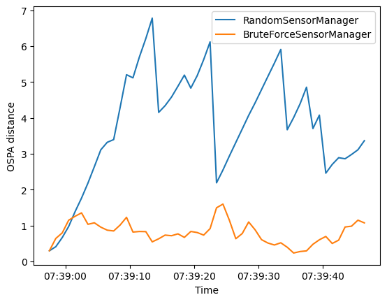
The BruteForceSensorManager generally results in a smaller OSPA distance than the random observations of the RandomSensorManager, reflecting the better tracking performance seen in the tracking plots.

SIAP metrics

Next we look at SIAP metrics. This can be done by generating a table which displays all the SIAP metrics computed, as seen in the Metrics Example. However, completeness, ambiguity and spuriousness are not relevant for this example because we are not initiating and deleting tracks and we have one track corresponding to each ground truth. Here we only plot positional accuracy and velocity accuracy over time.

fig, axes = plt.subplots(2)

times = metric_managerA.list_timestamps()

pa_metricA = metricsA['SIAP Position Accuracy at times']
va_metricA = metricsA['SIAP Velocity Accuracy at times']

pa_metricB = metricsB['SIAP Position Accuracy at times']
va_metricB = metricsB['SIAP Velocity Accuracy at times']

axes[0].set(title='Positional Accuracy', xlabel='Time', ylabel='PA')
axes[0].plot(times, [metric.value for metric in pa_metricA.value],
             label='RandomSensorManager')
axes[0].plot(times, [metric.value for metric in pa_metricB.value],
             label='BruteForceSensorManager')
axes[0].legend()

axes[1].set(title='Velocity Accuracy', xlabel='Time', ylabel='VA')
axes[1].plot(times, [metric.value for metric in va_metricA.value],
             label='RandomSensorManager')
axes[1].plot(times, [metric.value for metric in va_metricB.value],
             label='BruteForceSensorManager')
axes[1].legend()

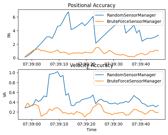
Similar to the OSPA distances the BruteForceSensorManager generally results in both a better positional accuracy and velocity accuracy than the random observations of the RandomSensorManager.

Uncertainty metric

Finally we look at the uncertainty metric which computes the sum of covariance matrix norms of each state at each time step. This is plotted over time for each sensor manager method.

uncertainty_metricA = metricsA['Sum of Covariance Norms Metric']
uncertainty_metricB = metricsB['Sum of Covariance Norms Metric']

fig = plt.figure()
ax = fig.add_subplot(1, 1, 1)
ax.plot([i.timestamp for i in uncertainty_metricA.value],
        [i.value for i in uncertainty_metricA.value],
        label='RandomSensorManager')
ax.plot([i.timestamp for i in uncertainty_metricB.value],
        [i.value for i in uncertainty_metricB.value],
        label='BruteForceSensorManager')
ax.set_ylabel("Sum of covariance matrix norms")
ax.set_xlabel("Time")
ax.legend()

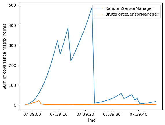
This metric shows that the uncertainty in the tracks generated by the RandomSensorManager is much greater than for those generated by the BruteForceSensorManager. This is also reflected by the uncertainty ellipses in the initial plots of tracks and truths.

References

[1]

Hero, A.O., Castanon, D., Cochran, D. and Kastella, K., Foundations and Applications of Sensor Management. New York: Springer, 2008.

[2]

D. Schuhmacher, B. Vo and B. Vo, A Consistent Metric for Performance Evaluation of Multi-Object Filters, IEEE Trans. Signal Processing 2008

[3]

Votruba, Paul & Nisley, Rich & Rothrock, Ron and Zombro, Brett., Single Integrated Air Picture (SIAP) Metrics Implementation, 2001