Note
Go to the end to download the full example code or to run this example in your browser via Binder
RangeRangeRateBinning measurement model example
RangeRangeRateBinning is a Cartesian to spherical measurement model. It takes a 6D
state of position and velocity in 3D Cartesian space and produces a 4D state of elevation
(\(\theta\)), bearing (\(\phi\)), range (\(r\)) and range-rate (\(\dot{r}\)),
This example demonstrates the RangeRangeRateBinning measurement model, showing the effect of binning
import numpy as np
from matplotlib import pyplot as plt
import datetime


# show and plot_states will help plot the results of RangeRangeRateBinning

def show(title='', x_label='', y_label=''):
    plt.minorticks_on()
    plt.grid(which='minor', alpha=0.2)
    plt.grid(which='major')
    plt.title(title, fontsize=15)
    plt.xlabel(x_label, fontsize=15)
    plt.ylabel(y_label, fontsize=15)
    plt.show()


def plot_states(state_vectors, mapping, plot=plt.plot, line='+-'):
    array = np.zeros([len(state_vectors), len(mapping)])
    for state_vector, index in zip(state_vectors, range(0, len(state_vectors))):
        for j in range(0, len(mapping)):
            array[index, j] = state_vector[mapping[j]]
    plot(array[:, 0], array[:, 1], line)
Measurement model
A measurement model is made with covariance of zero so that the effects of binning are more obvious.
from stonesoup.models.measurement.nonlinear import RangeRangeRateBinning
measurement_model = RangeRangeRateBinning(
    range_res=3,
    range_rate_res=1,
    ndim_state=6,
    mapping=[0, 2, 4],
    velocity_mapping=[1, 3, 5],
    noise_covar=np.diag([0., 0., 0., 0.]))
Create target
Then a target is created for the model to measure
from stonesoup.models.transition.linear import (CombinedLinearGaussianTransitionModel,
                                                ConstantVelocity)
from stonesoup.platform.base import MovingPlatform
from stonesoup.types.state import State

time_step = datetime.timedelta(seconds=0.1)
time_init = datetime.datetime.now()

transition_model = CombinedLinearGaussianTransitionModel(
    [ConstantVelocity(1.),
     ConstantVelocity(1.),
     ConstantVelocity(1.)])

red = MovingPlatform(
    position_mapping=[0, 2, 4],
    velocity_mapping=[0, 2, 4],
    states=State([50., 0., -50., 10., 0., 0.], timestamp=time_init),
    transition_model=transition_model)
Move target
Measure target states
The states are measured with and without noise to show the real position with the measured one.
measurements = []
noiseless_measurements = []
for state in red.states:
    measurements.append(measurement_model.function(state, noise=True))
    noiseless_measurements.append(measurement_model.function(state, noise=False))
Plot results
fig = plt.figure(figsize=[10, 10])
ax = fig.add_subplot(111, polar=True)
ax.set_thetamin(-60)
ax.set_thetamax(60)
ax.set_theta_zero_location('W', offset=-90)
plot_states(noiseless_measurements, [1, 2], plt.polar, 'r')
plot_states(measurements, [1, 2], plt.polar)
plt.legend(["real", "measured"])
plt.minorticks_on()
plt.title('Positions')
plt.grid(which='minor', alpha=0.2)
plt.show()
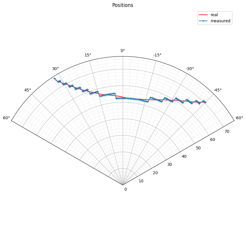
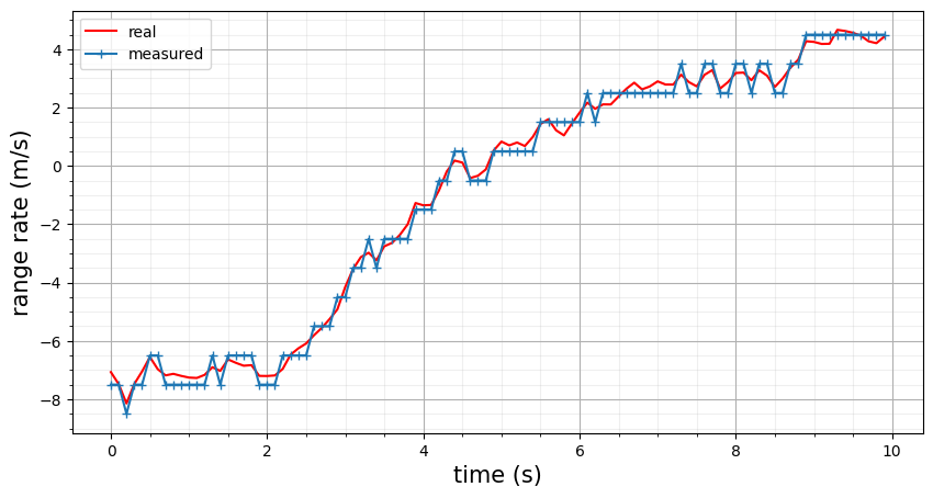
This graph shows the radial position is discrete. Next the velocity is plotted, showing the same binning but affecting the range rate
velocities = []
noiseless_velocities = []
for state_vector, noiseless in zip(measurements, noiseless_measurements):
    velocities.append(state_vector[3])
    noiseless_velocities.append(noiseless[3])

plt.figure(figsize=[10, 5])
plt.plot(np.arange(0, 100)*0.1, noiseless_velocities, 'r')
plt.plot(np.arange(0, 100)*0.1, velocities, '+-')
plt.legend(["real", "measured"])
show(x_label='time (s)', y_label='range rate (m/s)')
Total running time of the script: (0 minutes 1.234 seconds)