Metrics example

This example demonstrates some of the different metrics available in Stone Soup and how they can be used with the MultiManager to assess tracking performance. It also demonstrates how to use the MetricPlotter class to easily generate metric plots for visualisation.

To generate metrics, we need:

• At least one MetricGenerator - these are used to determine the metric type we want to generate and to compute the metrics themselves.

• The MultiManager metric manager - this is used to hold the metric generator(s) as well as all the ground truth, track, and detection sets we want to generate our metrics from. We will generate our metrics using the generate_metrics() method of the MultiManager class.

In this example, we will create a variety of metric generators for different types of metrics. These metrics will be used to assess and compare tracks produced from the same set of ground truth paths and detections by the Extended Kalman Filter and the Particle Filter.

Create metric generators and metric manager

In this section we create the metric generators in preparation for generating metrics later on.

First we create some Basic Metrics generators that will show us the number of tracks, the number of targets and the ratio of tracks to targets. As with all the metric generators, we must give our generator a unique name to identify it later, and the keys for our tracks and ground truth data (and detections set if relevant). When we generate the metrics, these keys will be used to access the data that we will store in the MultiManager and allow us to specify which tracks or truths we want to generate metrics for.

NB: in all metrics that take a track and a truth as input, it is possible to input two tracks instead for calculating track to track comparisons. This is relevant in scenarios where a second set of tracks is used as a proxy for ground truth. To do this, set the tracks_key parameter to the tracks set and the truths_key parameter to the second tracks set that is being used as a ground truth proxy.

from stonesoup.metricgenerator.basicmetrics import BasicMetrics

basic_EKF = BasicMetrics(generator_name='basic_EKF', tracks_key='EKF_tracks', truths_key='truths')
basic_PF = BasicMetrics(generator_name='basic_PF', tracks_key='PF_tracks', truths_key='truths')

Next we create the Optimal SubPattern Assignment (OSPA) metric generator. This metric is calculated at each time step to show how far the tracks are from the ground truth paths. It returns an overall multi-track to multi-ground-truth missed distance for each time step.

The generator has two additional properties: \(p \in [1,\infty]\) for outlier sensitivity and \(c > 1\) for cardinality penalty. [1]

from stonesoup.metricgenerator.ospametric import OSPAMetric

ospa_EKF_truth = OSPAMetric(c=40, p=1, generator_name='OSPA_EKF-truth',
                            tracks_key='EKF_tracks', truths_key='truths')
ospa_PF_truth = OSPAMetric(c=40, p=1, generator_name='OSPA_PF-truth',
                           tracks_key='PF_tracks', truths_key='truths')
ospa_EKF_PF = OSPAMetric(c=40, p=1, generator_name='OSPA_EKF-PF',
                         tracks_key='EKF_tracks', truths_key='PF_tracks')

Next we create the Single Integrated Air Picture (SIAP) metric generators. These metrics are applicable to tracking in general and not just in relation to an air picture. [2]

The SIAP generators will generate a series of different individual SIAP metrics that will provide information about the accuracy of the tracking. They will generate different SIAP metrics for each time step, as well as overall averages. You will see the SIAP metric averages and more detail about what the different metrics mean in the table generated towards the end of the notebook.

The SIAP Metrics require a way to associate tracks to truth, so we’ll use a Track to Truth associator which uses Euclidean distance measure by default.

from stonesoup.metricgenerator.tracktotruthmetrics import SIAPMetrics
from stonesoup.measures import Euclidean

siap_EKF_truth = SIAPMetrics(position_measure=Euclidean((0, 2)),
                             velocity_measure=Euclidean((1, 3)),
                             generator_name='SIAP_EKF-truth',
                             tracks_key='EKF_tracks',
                             truths_key='truths'
                             )

siap_PF_truth = SIAPMetrics(position_measure=Euclidean((0, 2)),
                            velocity_measure=Euclidean((1, 3)),
                            generator_name='SIAP_PF-truth',
                            tracks_key='PF_tracks',
                            truths_key='truths'
                            )

from stonesoup.dataassociator.tracktotrack import TrackToTruth

associator = TrackToTruth(association_threshold=30)

Next we create metric generators for the Sum of Covariance Norms. They will calculate the sum of the covariance matrix norms of each track state at each time step. These metrics produced will indicate how uncertain the tracks we have produced are. Higher sum of covariance norms means higher uncertainty.

from stonesoup.metricgenerator.uncertaintymetric import SumofCovarianceNormsMetric

sum_cov_norms_EKF = SumofCovarianceNormsMetric(tracks_key='EKF_tracks',
                                               generator_name='sum_cov_norms_EKF')
sum_cov_norms_PF = SumofCovarianceNormsMetric(tracks_key='PF_tracks',
                                              generator_name='sum_cov_norms_PF')

Finally, we create two plot generators - one for each of the two different trackers we are using. These will take in the tracks, ground truths, and detections that we generate and plot them in 2 dimensions.

from stonesoup.metricgenerator.plotter import TwoDPlotter

plot_generator_EKF = TwoDPlotter([0, 2], [0, 2], [0, 2], uncertainty=True, tracks_key='EKF_tracks',
                                 truths_key='truths', detections_key='detections',
                                 generator_name='EKF_plot')
plot_generator_PF = TwoDPlotter([0, 2], [0, 2], [0, 2], uncertainty=True, tracks_key='PF_tracks',
                                truths_key='truths', detections_key='detections',
                                generator_name='PF_plot')

Now we add all of our metric generators to the MultiManager.

from stonesoup.metricgenerator.manager import MultiManager

metric_manager = MultiManager([basic_EKF,
                               basic_PF,
                               ospa_EKF_truth,
                               ospa_PF_truth,
                               ospa_EKF_PF,
                               siap_EKF_truth,
                               siap_PF_truth,
                               sum_cov_norms_EKF,
                               sum_cov_norms_PF,
                               plot_generator_EKF,
                               plot_generator_PF
                               ], associator)  # associator for generating SIAP metrics

Generate ground truth and detections

In this section, we generate the ground truth paths and the detections to be tracked - we will simulate targets that can turn left or right. Both our Extended Kalman Filter tracker and Particle Filter tracker will be given the same sets of truths and detections to track so that we can fairly compare the results.

import numpy as np
import datetime
from stonesoup.types.array import StateVector, CovarianceMatrix
from stonesoup.types.state import State, GaussianState

start_time = datetime.datetime.now()
np.random.seed(8)
initial_state_mean = StateVector([[0], [0], [0], [0]])
initial_state_covariance = CovarianceMatrix(np.diag([4, 0.5, 4, 0.5]))
timestep_size = datetime.timedelta(seconds=5)
number_steps = 20
initial_state = GaussianState(initial_state_mean, initial_state_covariance)

from stonesoup.models.transition.linear import \
    CombinedLinearGaussianTransitionModel, ConstantVelocity, KnownTurnRate

# initialise the transition models the ground truth can use
constant_velocity = CombinedLinearGaussianTransitionModel(
    [ConstantVelocity(0.05), ConstantVelocity(0.05)])
turn_left = KnownTurnRate([0.05, 0.05], np.radians(20))
turn_right = KnownTurnRate([0.05, 0.05], np.radians(-20))

# create a probability matrix - how likely the ground truth will use each transition model,
# given its current model
model_probs = np.array([[0.7, 0.15, 0.15],  # keep straight, turn left, turn right
                        [0.4, 0.6, 0.0],  # go straight, keep turning left, turn right
                        [0.4, 0.0, 0.6]])  # go straight, turn left, keep turning right

from stonesoup.simulator.simple import SwitchMultiTargetGroundTruthSimulator
from stonesoup.types.state import GaussianState

# generate truths
n_truths = 3
xmin = 0
xmax = 40
ymin = 0
ymax = 40
preexisting_states = []

for i in range(0, n_truths):
    x = np.random.randint(xmin, xmax) - 1  # x position of initial state
    y = np.random.randint(ymin, ymax) - 1  # y position of initial state
    x_vel = np.random.randint(-20, 20) / 10  # x velocity will start between -2 and 2
    y_vel = np.random.randint(-20, 20) / 10  # y velocity will start between -2 and 2
    preexisting_states.append(StateVector([x, x_vel, y, y_vel]))

ground_truth_gen = SwitchMultiTargetGroundTruthSimulator(
    initial_state=initial_state,
    transition_models=[constant_velocity, turn_left, turn_right],
    model_probs=model_probs,  # put in matrix from above
    number_steps=number_steps,  # how long we want each track to be
    birth_rate=0,
    death_probability=0,
    preexisting_states=preexisting_states
)

Next we create a sensor and use it to generate detections from the targets. The sensor we use in this example is a radar with imperfect measurements in bearing-range space.

from stonesoup.sensor.radar import RadarBearingRange

# Create the sensor
sensor = RadarBearingRange(
    ndim_state=4,
    position_mapping=[0, 2],  # Detecting x and y
    noise_covar=np.diag([np.radians(0.2), 0.2]),  # Radar doesn't take perfect measurements
    clutter_model=None,  # Can add clutter model in future if desired
)

from stonesoup.platform import FixedPlatform

platform = FixedPlatform(State(StateVector([20, 0, 0, 0])), position_mapping=[0, 2],
                         sensors=[sensor])

# create identical detection sets for each tracker to use
from itertools import tee
from stonesoup.simulator.platform import PlatformDetectionSimulator

detector = PlatformDetectionSimulator(ground_truth_gen, platforms=[platform])
detector, *detectors = tee(detector, 3)

Now we plot the ground truth paths and detections:

detections = set()
truths = set()

for time, detects in detector:
    detections |= detects
    truths |= ground_truth_gen.groundtruth_paths

from stonesoup.plotter import Plotterly

plotter = Plotterly()
plotter.plot_ground_truths(truths, [0, 2])
plotter.plot_measurements(detections, [0, 2])
plotter.plot_sensors(sensor)
plotter.fig

Create and run the trackers

Now we create and run the two different trackers, one with the Extended Kalman Filter (EKF) and one with the Particle Filter (PF). We start first with the EKF tracker.

from stonesoup.predictor.kalman import ExtendedKalmanPredictor
from stonesoup.updater.kalman import ExtendedKalmanUpdater

transition_model_estimate = CombinedLinearGaussianTransitionModel([ConstantVelocity(0.5),
                                                                   ConstantVelocity(0.5)])
predictor_EKF = ExtendedKalmanPredictor(transition_model_estimate)
updater_EKF = ExtendedKalmanUpdater(sensor)

from stonesoup.hypothesiser.distance import DistanceHypothesiser
from stonesoup.measures import Mahalanobis

hypothesiser_EKF = DistanceHypothesiser(predictor_EKF, updater_EKF,
                                        measure=Mahalanobis(), missed_distance=4)

from stonesoup.dataassociator.neighbour import GNNWith2DAssignment

data_associator_EKF = GNNWith2DAssignment(hypothesiser_EKF)

from stonesoup.deleter.time import UpdateTimeDeleter

deleter = UpdateTimeDeleter(datetime.timedelta(seconds=5), delete_last_pred=True)

init_transition_model = CombinedLinearGaussianTransitionModel(
    (ConstantVelocity(1), ConstantVelocity(1)))
init_predictor_EKF = ExtendedKalmanPredictor(init_transition_model)

from stonesoup.initiator.simple import MultiMeasurementInitiator

initiator_EKF = MultiMeasurementInitiator(
    GaussianState(
        np.array([[20], [0], [10], [0]]),  # Prior State
        np.diag([1, 1, 1, 1])),
    measurement_model=None,
    deleter=deleter,
    data_associator=GNNWith2DAssignment(
        DistanceHypothesiser(init_predictor_EKF, updater_EKF, Mahalanobis(), missed_distance=5)),
    updater=updater_EKF,
    min_points=2
)

from stonesoup.tracker.simple import MultiTargetTracker

kalman_tracker_EKF = MultiTargetTracker(  # Runs the tracker
    initiator=initiator_EKF,
    deleter=deleter,
    detector=detectors[0],
    data_associator=data_associator_EKF,
    updater=updater_EKF
)

Now we create and run the tracker with the Particle Filter:

from stonesoup.predictor.particle import ParticlePredictor
from stonesoup.resampler.particle import ESSResampler

resampler = ESSResampler()
from stonesoup.updater.particle import ParticleUpdater

predictor_PF = ParticlePredictor(transition_model_estimate)
updater_PF = ParticleUpdater(measurement_model=None, resampler=resampler)

hypothesiser_PF = DistanceHypothesiser(predictor_PF, updater_PF,
                                       measure=Mahalanobis(), missed_distance=4)
data_associator_PF = GNNWith2DAssignment(hypothesiser_PF)

init_predictor_PF = ParticlePredictor(init_transition_model)

from stonesoup.initiator.simple import GaussianParticleInitiator
from stonesoup.types.state import GaussianState
from stonesoup.initiator.simple import SimpleMeasurementInitiator

prior_state = GaussianState(
    StateVector([20, 0, 10, 0]),
    np.diag([1, 1, 1, 1]) ** 2)

initiator_Part = SimpleMeasurementInitiator(prior_state, measurement_model=None,
                                            skip_non_reversible=True)
initiator_PF = GaussianParticleInitiator(number_particles=2000,
                                         initiator=initiator_Part,
                                         use_fixed_covar=False)

tracker_PF = MultiTargetTracker(
    initiator=initiator_PF,
    deleter=deleter,
    detector=detectors[1],
    data_associator=data_associator_PF,
    updater=updater_PF,
)

Add data to metric manager and generate metrics

Now that we have all of our ground truth, detections, and tracks data, we can add it to the metric manager.

The MultiManager add_data() method takes a dictionary of lists/sets of ground truth, detections, and/or tracks data. It can take multiple sets of each type. Each state set must have a unique key assigned to it. The track, truth, and detection keys that we input into the metric generators will be used to extract the corresponding set from the MultiManager for metric generation.

Setting overwrite to False allows new data to be added to the MultiManager without overwriting data that is already in it, as demonstrated in the code below.

# add tracks data to metric manager
for step, (time, current_tracks) in enumerate(kalman_tracker_EKF, 1):
    metric_manager.add_data({'EKF_tracks': current_tracks}, overwrite=False)

for step, (time, current_tracks) in enumerate(tracker_PF, 1):
    metric_manager.add_data({'PF_tracks': current_tracks}, overwrite=False)

# then add truths and detections
metric_manager.add_data({'truths': truths,
                         'detections': detections}, overwrite=False)

Generate metrics

We are now ready to generate and view all the metrics from our MultiManager.

Because we have two plot generators in our metric manager, two plots will be produced and displayed when we generate the metrics. They will show the ground truth paths, detections, and tracks. One will display the tracks produced by the EKF tracker and the other will display the tracks from the PF tracker.

metrics = metric_manager.generate_metrics()

• 
• 

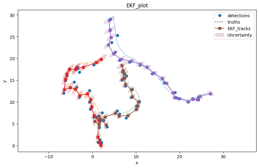
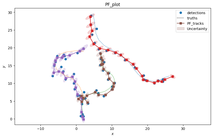
We can see from the plots above that the two trackers exhibit similar performance in tracking the ground truths.

Let’s look at the metrics we’ve generated to compare them further. We’ll start by printing out the basic metrics, which give us information on the number of tracks versus targets.

for generator in metrics.keys():
    if 'basic' in generator:
        print(f'\n{generator}:')
        for metric_key, metric in metrics[generator].items():
            print(f"{metric.title}: {metric.value}")

basic_EKF:
Number of targets: 3
Number of tracks: 3
Track-to-target ratio: 1.0

basic_PF:
Number of targets: 3
Number of tracks: 3
Track-to-target ratio: 1.0

The basic metrics show that both the EKF and the PF have successfully produced tracks for each of the ground truth paths so have a 1:1 track-to-target ratio.

Next we’ll look at the averages of each of the SIAP metrics to compare.

First we extract the SIAP averages from the MultiManager. Then we use the SIAPTableGenerator to display the average metrics in a table which shows us descriptions for each metric.

We will create a table for the EKF SIAPs first.

from stonesoup.metricgenerator.metrictables import SIAPTableGenerator

siap_metrics = metrics['SIAP_EKF-truth']
siap_averages_EKF = {siap_metrics.get(metric) for metric in siap_metrics
                     if metric.startswith("SIAP") and not metric.endswith(" at times")}
siap_table = SIAPTableGenerator(siap_averages_EKF).compute_metric()

Now we produce a table for the PF SIAPs for comparison.

siap_metrics = metrics['SIAP_PF-truth']
siap_averages_PF = {siap_metrics.get(metric) for metric in siap_metrics
                    if metric.startswith("SIAP") and not metric.endswith(" at times")}
siap_table = SIAPTableGenerator(siap_averages_PF).compute_metric()

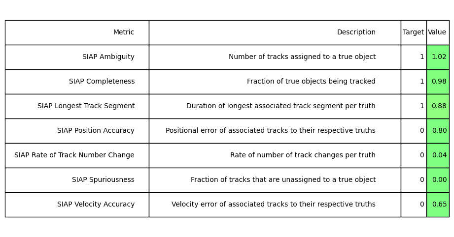
We can see that the values for most of the SIAP metric averages are not very different between the two trackers, again showing their tracking quality is very similar. Other specific observations include:

• SIAP Ambiguity of just above 1 indicates that there are places where multiple tracks overlap the same section of ground truth path, which we can see is the case from the plots above.

• A Longest Track Segment of 0.88 indicates that on average the three different tracks produced are not following 100% of the ground truth paths. We can see on the lower left area of our plots that the tracks have been confused.

• Positional and velocity errors of ~0.80 and 0.66, respectively, indicate that there is some distance between the tracks and ground truth paths. Again, we can see this from the plots. The range for these errors is 0-infinity so the errors are not significant.

• SIAP Spuriousness of 0 show us no tracks have been created that are not associated to a true object. We might get higher spuriousness if we added clutter to our detections.

Plot metrics

We will use MetricPlotter to plot some of our metrics below.

To use MetricPlotter we first create an instance of the class. We can then use the plot_metrics() method to plot the metrics of our choice. Key features of MetricPlotter:

• You can specify exactly which metrics you want to plot by specifying the optional generator_names and metric_names parameters.

• generator_names allows you to specify which generators you want to plot metrics from. If you don’t pass the generator_names argument, plot_metrics() will automatically extract all plottable metrics from all metric generators in the MultiManager and plot them.

• metric_names allows you to specify which specific metrics types you want to plot from the metric generators. This is mostly relevant for the SIAP metrics. You can view which metrics are plottable with MetricPlotter.plottable_metrics().

• plot_metrics() has a combine_plots argument which defaults to True. This means that all metrics of the same type will be plotted together on a single subplot.

• You can specify additional formatting, like colour and linestyle, for the plots produced by using keyword arguments from matplotlib pyplot.

We start by plotting the OSPA distances and SIAP metrics. Plots will be combined for the same metric type.

from stonesoup.plotter import MetricPlotter

graph = MetricPlotter()
graph.plot_metrics(metrics, generator_names=['OSPA_EKF-truth',
                                             'OSPA_PF-truth',
                                             'OSPA_EKF-PF',
                                             'SIAP_EKF-truth',
                                             'SIAP_PF-truth'],
                   # metric_names=['OSPA distances',
                   #               'SIAP Position Accuracy at times'],  # uncomment and run to see effect
                   color=['orange', 'green', 'blue'])

# update y-axis label and title, other subplots are displaying auto-generated title and labels
graph.axes[0].set(ylabel='OSPA metrics', title='OSPA distances over time')
graph.fig.show()

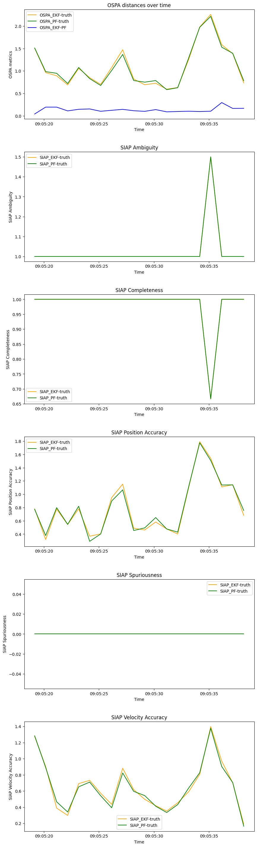
From these plots, we can see that towards the end of the time frame is where we lose some accuracy of our tracks and where more errors are introduced. We can once again see how similar the tracking performance is across both trackers. The blue line in the OSPA distances plot indicates the distance between tracks produced by both trackers at each time step.

Now we will plot the sum of covariance norms metrics for both trackers. This time we plot the metrics separately and we specify additional keyword arguments to customise the plot.

graph = MetricPlotter()
graph.plot_metrics(metrics, generator_names=['sum_cov_norms_EKF',
                                             'sum_cov_norms_PF'],
                   combine_plots=False,
                   color='purple', linestyle='--')
graph.set_fig_title('Sum of Covariance Norms Metric')  # set figure title
graph.set_ax_title(['Extended Kalman Filter', 'Particle Filter'])  # set title for each axis

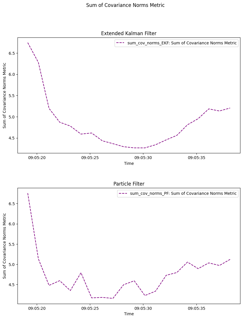
For both trackers, we start with the highest uncertainty as tracks are initiated. Uncertainty decreases until just past the middle of our timeframe and begins to increase again as we get further from the start time.

You can change the parameters in the ground truth and trackers and see how it affects the different metrics.

Footnotes

[1]

D. Schuhmacher, B. Vo and B. Vo, A Consistent Metric for Performance Evaluation of Multi-Object Filters, IEEE Trans. Signal Processing 2008

[2]

Karoly S., Wilson J., Dutchyshyn H., Maluda J., Single Integrated Air Picture (SIAP) Attributes Version 2.0, DTIC Technical Report 2003